Computed Tomography Kidney Disease Recognition using Deep Learning

Abstract

The present paper demonstrates kidney disease recognition in computed tomography (CT) images using deep neural networks, including convolutional neural networks (CNNs), the visual geometry group (VGG) network, and the deep residual network (ResNet-50). The kidney disease dataset consists of images among four categories, i.e cyst, normal, stone, and tumor. The class “cyst” consists of 3,709 images, the class “normal” consists of 5,077 images, the class “stone” consists of 1,377 images, and finally the class “tumor” consists of 2,283 images. In total, the dataset has 12,446 images. This dataset was passed through the deep CNN, VGG19, and ResNet-50 models to obtain the results. The major novelty of this work compared to previous works is that the algorithms of the CNN and ResNet-50 models have been modified, compared to existing works. The results, such as error/positive-predictive-value (PPV), error/probability of detection (POD), and error/area under the curve (AUC) curves, are shown for the confirmation of the work. Further, the error matrix, specificity/POD, and PPV/POD curves are also shown for the justification of the work. Finally, the performance metrics such as accuracy, PPV, POD, and F1-score values obtained from the error matrix are also shown for the justification of the work. The CNN model has achieved an accuracy of 0.95 for class “cyst”, 0.82 for class “normal”, 0.89 for class “stone”, and 0.87 for class “tumor”. The VGG19 neural network model has achieved an accuracy of 0.95 for class “cyst”, 0.79 for class “normal”, 0.84 for class “stone”, and 0.89 for class “tumor”. The ResNet-50 neural network model has achieved an accuracy of 0.92 for class “cyst”, 0.82 for class “normal”, 0.84 for class “stone”, and 0.92 for class “tumor”. The deep CNN model has achieved an area under the curve (AUC) value of 0.98 for class “cyst”, 0.87 for class “normal”, 0.92 for class “stone”, and 0.91 for class “tumor”. The deep CNN model has the highest AUC value for class “cyst” compared to other classes. The VGG19 model has an AUC value of 0.99 for class “cyst”, 0.92 for class “normal”, 1.00 for class “stone”, and 0.96 for class “tumor”. The VGG19 model has the highest AUC value for class “stone” compared to other classes. The ResNet-50 model has AUC values of 0.96 for class “cyst”, 0.92 for class “normal”, 0.92 for class “stone”, and 0.86 for class “tumor”. The ResNet-50 model has the highest AUC value for class “cyst” compared to the other classes.

Introduction

Deep learning is a branch of artificial intelligence that consists of several deep neural networks such as convolutional neural network (CNN), Alex network, and visual geometry group (VGG)-19 layer neural network. These networks have been found in various medical imaging applications such as kidney disease recognition [1], brain-tumor recognition [2], heart-attack-analysis-prediction [3], and so on. Here, kidney disease recognition has been considered a major issue that has been performed using deep learning neural networks such as deep CNN, VGG19, and ResNet-50.

Kidney disease represents a critical global public health challenge, with its incidence rising steadily despite sustained prevention and management strategies [4]. Chronic kidney disease (CKD) affects over 10% of the global population. In 2016, CKD was ranked as the 16th leading cause of death worldwide and is projected to escalate to the 5th leading cause by 2040, underscoring its growing burden on healthcare systems [5,6]. Apart from chronic kidney disease, several other renal disorders—namely cyst formation, nephrolithiasis (kidney stones), and renal cell carcinoma (RCC)—are frequently encountered and significantly compromise kidney function. A kidney cyst is a fluid-filled sac that develops on the surface of the kidney and is typically encapsulated by a thin wall. Single or multiple cysts may arise within the renal parenchyma, usually demonstrating water density values ranging from 0 to 20 Hounsfield units (HU) in computed tomography (CT) imaging [7-9]. Nephrolithiasis is characterized by the formation of crystalline mineral concretions within the kidneys and affects nearly 12% of the global population [10]. Renal cell carcinoma, commonly referred to as a kidney tumor, ranks among the ten most prevalent malignancies worldwide, highlighting its substantial clinical significance [11]. Diagnostic imaging modalities—including X-ray, computed tomography (CT), B-ultrasound (US), and magnetic resonance imaging (MRI)—are extensively utilized, often alongside histopathological examinations, for the accurate identification of kidney diseases. Nevertheless, the availability of specialized healthcare professionals remains critically inadequate. The global workforce of nephrologists and radiologists is insufficient to meet the rising clinical demand [12]. In South Asia, there is approximately one nephrologist per million population, in stark contrast to Europe, where the density ranges from 22.9 to 25.7 nephrologists per million people. Considering the escalating burden of kidney diseases, the pronounced shortage of expert clinicians worldwide, and the rapid progress of deep learning techniques in medical image analysis, the development of artificial intelligence (AI)–driven systems has become essential. Such models can facilitate automated detection of renal radiological abnormalities, support clinical decision-making, and ultimately help reduce patient morbidity through timely and accessible diagnosis.

Wasi et.al performed kidney tumor recognition for abdominal CT images using a VGG-16 layer neural network [13]. In this work, the binary classification of kidney disease images between kidney and tumor images was performed using a VGG-16 layer neural network. The VGG-16 layer neural network achieves an accuracy of 0.92, PPV of 0.80, POD of 0.93, and F1-score of 0.86. Anuruk Prommakhot et.al performed kidney tumor classification for computed tomography images using a VGG-16 layer neural network [14]. In this work, the multi-class classification of kidney disease images, such as class “cyst”, class “normal”, class “stone”, and class “tumor”, was performed using a VGG-16 layer neural network. Brehar et.al performed kidney-tumor segmentation and grade identification in computed tomography images using various deep learning neural network models [15]. This research work is related to kidney tumor segmentation, and here no classification task has been performed among classes “cyst”, “normal”, “stone”, and “tumor”. Yang et.al performed automatic segmentation of kidney and renal tumor in CT images using a deep CNN and pyramid pooling module [16]. Here, in this research work, the classification of kidney disease images such as “cyst”, “normal”, “stone”, and “tumor” has not been performed. Zhao et.al performed kidney tumor segmentation using boundary attention U-Net [17]. Here also, this research work is related to kidney tumor segmentation performed using boundary attention U-Network. Islam et.al used vision transformers and explainable transfer learning models for auto-detection of kidney disease images, namely cyst, normal, stone, and tumor images [18]. In this research work, the multi-class classification of kidney disease images such as class “cyst”, class “normal”, class “stone”, and class “tumor” has been performed using various deep neural network models such as VGG16, ResNet50, InceptionV3, Swin Transformer, and compact convolutional transformer (CCT) neural network models. The performance metrics such as accuracy, PPV, POD, and F1-score values have been compared among these neural network models. Alzu’bi. et.al proposed kidney tumor detection and classification using deep CNN, VGG16, and ResNet50 models [19]. In this research work, the multi-class classification of kidney disease images such as cyst, normal, stone, and tumor was performed using 2D CNN-six layer, 2D CNN-four layer, and ResNet50 neural network models. The performance metrics such as accuracy, PPV, POD, and F1-score were compared among these three neural network models. Hossain MN, et al. performed detection and classification of kidney disease images using hybrid deep learning models such as DenseNet-121 and EfficientNet-B0 models which were used for feature extraction followed by Support Vector Machine (SVM), Random-Forest, and XGBoost Classifiers used for classification of cyst, normal, stone, and tumor images [20]. Fariha Jahan, et al. performed kidney segmentation and classification from computed tomography (CT) images using a modified U-Net model and EfficientNet-B3 model. The modified U-Net model was used for segmentation purposes, with results such as accuracy, Dice coefficient, and intersection over union (IOU) metrics approaching around 98%. The classification of CT images among four categories was also performed, including cyst, normal, stone, and tumor, using the EfficientNetB3 model with accuracy approaching around 99.3% [21]. Yogesh Kumar et.al performed classification of kidney disease images among four categories, such as cyst, normal, stone, and tumor images, using pre-trained deep learning neural network models such as DenseNet-201, EfficientNetB0, InceptionResNetV2, MobileNetV2, ResNet50V2, and Xception models among three different optimizers, such as Root Mean Square(RMS) propagation, Stochastic Gradient Descent (SGD), and Adam. Among these several neural network models, the Xception model performed best with an accuracy of 99.8% using the RMS propagation optimizer. Similarly, ResNet50V2 and DenseNet201 models demonstrated accuracy of 99.6% using SGD and Adam optimizers [22]. Niharika Vemula, et al. performed kidney disease detection and classification of CT images among four categories such as cyst, normal, stone, and tumor using a pre-trained deep learning neural network model such as ResNet-50 with hybrid activation functions such as ReLU, Swish, ELU, Mish, and Hard Swish. The proposed model trained with several activation functions produced the highest accuracy of 95% when Mish+ELU+HardSwish (Hybrid) activation functions are combined [23].

The present paper describes the computed tomography kidney disease recognition for four classes, namely class “cyst”, “normal”, “stone”, and “tumor,” using deep CNN, VGG19, and ResNet-50 layer neural network models. The dataset consisting of four classes of images was passed through deep CNN, VGG19, and ResNet-50 layer neural network models to produce the results. The results, such as loss/positive-predictive-value (PPV)/probability of detection (POD)/area under the curve (AUC) curves on training and validation sets, are shown for the confirmation of the work [25, 27-35]. Further, the results such as error matrix, specificity/POD, and PPV/POD curves are shown for the justification of the work [25, 27-35]. Finally, the performance metrics such as accuracy, PPV, POD, and F1-score values obtained from the error matrix are also shown for the justification of the work. The proposed deep neural network models have already been used on the existing dataset, but the major difference is that the proposed algorithm of deep CNN, VGG19 neural network, and ResNet-50 neural network models has provided better results compared to earlier works [13,14,18-19].

Methodology

In this section, the architectures of the deep CNN, VGG19, and ResNet-50 for kidney disease recognition are discussed.

(A) Convolutional Neural Network (CNN)

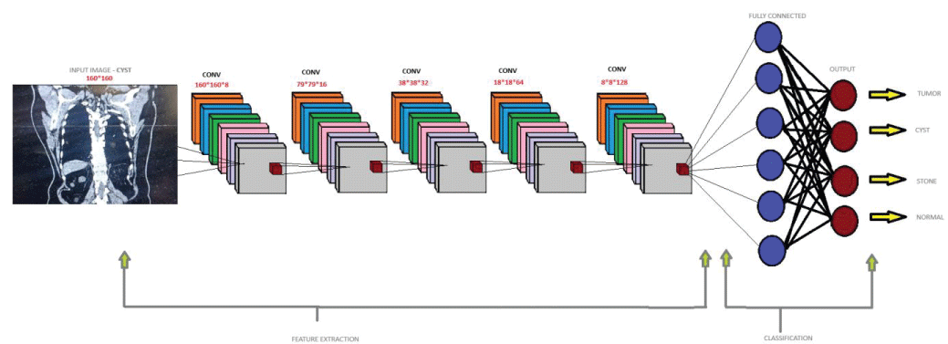
The architecture of the deep CNN for kidney disease recognition is shown in Figure 1. The deep CNN accepts kidney disease image of size 160 × 160 from 705 × 569/512 × 512.

Figure 1: Block diagram of Convolutional Neural Network (CNN).

The deep CNN consists of five stages of convolutional and pooling layers for feature extraction. The convolutional layer performs a convolution operation between the kidney disease image and the kernel to produce the feature map. The output of the convolutional layer is given by

$C_{ab}^{\left(k\right)}=T({\Sigma }_{m=0}^p{\Sigma }_{n=0}^p{E}_{mn}^{(k)}{A}_{ab}+D_{ab}).$ (1)

In the eqn. (1), represents the output of the convolutional layer and Aab represents the input kidney disease image, represents kernel values, k represents the number of kernels, p represents the kernel size, T represents the Rectified Linear Unit (ReLU) activation function, and Dab represents bias [25,27-35]. The values of k in the respective convolutional layers are 8, 16, 32, 64, and 128. i.e the first convolutional layer incorporates 8 kernels, the second convolutional layer incorporates 16 kernels, the third convolutional layer incorporates 32 kernels, the fourth convolutional layer incorporates 64 kernels, and the fifth convolutional layer incorporates 128 kernels. The value of p is 3 × 3. i.e the kernel size in all convolutional layers used is 3 × 3. All five convolutional layers incorporate the ReLU activation function. The stride is 1 in all five convolutional layers, and no padding is used in any of them. The output of each convolutional layer is passed through the subsequent pooling layer. The pooling technique employed was Max-Pooling2D. The output of the Max-Pooling2D is given by

$M_{ab}=\text{max}(N_{ab})$ (2)

In the eqn. (2), Mab represents the output and Nab represents the input [25,27-35]. The input to the first convolutional layer is 160 × 160 × 8. The output of the first convolutional layer is 158 × 158 × 8. The output of the first convolutional layer is passed as input to the first pooling layer. The first pooling layer takes an input dimension of 158 × 158 × 8 and produces an output dimension of 79 × 79 × 8. Like this, the same process is repeated for four more stages. The model summary of the deep CNN model used for kidney disease recognition is shown in Table 1. Table 1 describes the dimensions of input and output in each of the convolutional and pooling layers. The input to the fifth convolutional layer is 8 × 8 × 128. The output of the fifth convolutional layer is 6 × 6 × 128. The output of the fifth convolutional layer is passed through the final/fifth pooling layer. The fifth pooling layer takes input dimension of 6 × 6 × 128 and produces an output dimension of 3 × 3 × 128. The output of the final pooling layer is flattened and given to the fully connected layer to produce the result. The output of the fully connected layer is given by

$C_q=T({\Sigma }_{q=1}^z{F}_{xy}{A}_q+D_q)$ (3)

In the eqn. (3), Cq represents the output and Dq represents the bias, T represents the ReLU activation function, Fxy represents weight values, Aq represents the one dimensional (1-D) data obtained through the flatten layer, and z represents the number of neurons [25,27-35]. The final/fifth pooling layer output i.e 3 × 3 × 128 is flattened to produce 1152 neurons. The fully connected layer selects 16 neurons among 1152 neurons. i.e the value of z is 16. The output of the fully connected layer is given to the output layer to perform the kidney disease recognition task. The output layer consists of 4 neurons along with the softmax activation function to produce the result. The expression for the softmax activation function is shown below in eqn. (4).

$A_k=\frac{\text{exp}(C_k)}{{{\displaystyle \sum }}_{l=1}^Q\text{exp}(C_l)}$ (4)

In the eqn. (4), where Ak represents the output, Ck represents the input, and Q represents the number of neurons [25,27-35]. Four neurons are considered in the output layer because four-class classification of kidney disease images has been performed. i.e multi-class classification of kidney disease images cyst, normal, stone, and tumor categories was performed. The expressions (1-2) represent the equations for convolutional and pooling layers. The expressions (3-4)

represent the equations for the fully connected layer and softmax activation functions.

(B) VGG19 neural network

The architecture of the Visual Geometry Group (VGG-19) layer neural network for kidney disease recognition is shown in Figure 2. The VGG-19 layer neural network accepts kidney disease image of size 224 × 224 from 705 × 569/512 × 512. The VGG-19 layer neural network consists of sixteen convolutional layers, five pooling layers, and three fully connected layers. The convolutional layers use k values of 64 (Layers 1–2), 128 (Layers 3–4), 256 (Layers 5–8), and 512 (Layers 9–16). i.e the number of kernels in the first and second convolutional layers is 64. The number of kernels in the third and fourth convolutional layers is 128. The number of kernels in the fifth, sixth, seventh, and eighth convolutional layers is 256. The number of kernels in the ninth, tenth, eleventh, twelfth, thirteenth, fourteenth, fifteenth, and sixteenth convolutional layers is 512. A uniform kernel size (p) of 3 × 3 is adopted across all convolutional layers. Max-pooling layers are placed between the convolutional layers. Two dense layers are employed, each with 4096 neurons. The fully connected layer output is forwarded to the output layer for kidney disease recognition. The output layer contains four neurons with a softmax activation function. The model summary of the VGG-19 layer neural network is shown in Table 2. The VGG19 is a pre-trained neural network model with weights obtained from convolutional layers and further the output of the convolutional layer is passed through the subsequent pooling layers. Here, stride=1, and “padding=same” condition is applied in all convolutional layers to maintain the same dimension of input and output feature maps. The input and output dimensions of each of the convolutional and pooling layers are shown in Table 2.

Figure 2: Block diagram of VGG19 neural network.

(C) ResNet-50 deep neural network

The ResNet50 model [24] requires input images of size 64 × 64 pixels. Therefore, the original kidney disease images, which have dimensions of either 705 569pixels or 512 × 512 pixels, are resized to 64 × 64 pixels prior to being provided as input to the network. This preprocessing step ensures that all images conform to the required input dimensions of the ResNet50 architecture while maintaining a consistent format for model training and evaluation. The ResNet50 model consists of 50 layers and incorporates several key components, including convolutional layers, batch normalization layers, pooling layers, residual blocks, and activation functions. The residual learning architecture enables the network to effectively learn deep feature representations while mitigating the vanishing-gradient problem associated with conventional deep neural networks. In ResNet50, the ReLU activation function is employed to introduce non-linearity into the network and facilitate the learning of complex feature representations. The network incorporates residual blocks with skip connections, which allow the input of a block to bypass one or more convolutional layers and be directly added to the block output. These residual connections facilitate the propagation of gradients through the deeper network and help alleviate the vanishing-gradient problem. The convolutional layers perform convolution operations between the input image and learnable kernels to generate feature maps containing relevant spatial features. The extracted feature maps are subsequently processed through pooling operations to reduce their spatial dimensions and computational complexity while retaining the most prominent features. Batch normalization is applied within the network to normalize the intermediate feature representations, thereby improving training stability and accelerating convergence. The ResNet50 architecture comprises multiple stages of residual blocks, with different stages containing three, four, six, and three bottleneck blocks, respectively. The combination of convolutional layers, batch normalization, ReLU activation, pooling operations, and residual connections enables ResNet50 to effectively extract hierarchical and discriminative features from kidney disease images. The first convolutional layer (convolutional layer1) consists of three residual blocks each with 1 × 1, 3 × 3, and 1 × 1 convolutional layers. The first convolutional layer is followed by batch normalization and ReLU activation, while the residual blocks incorporate skip connections to facilitate the propagation of information and gradients through the network. The second, third, and fourth residual stages of the ResNet50 architecture comprise four, six, and three residual blocks, respectively. These residual stages employ convolutional kernels with different dimensions and numbers of filters to progressively extract higher-level and more discriminative features from the input kidney disease images. The output feature maps obtained from the final residual stage are subsequently transformed into a one-dimensional feature vector and passed to the fully connected layer for classification. The final output layer consists of four neurons corresponding to the four kidney disease classes and employs the Softmax activation function to generate the class probabilities. The architectural details and layer-wise configuration of the ResNet50 (deep residual network) model used in this study are presented in Table 3.

Dataset preparation and results and discussions

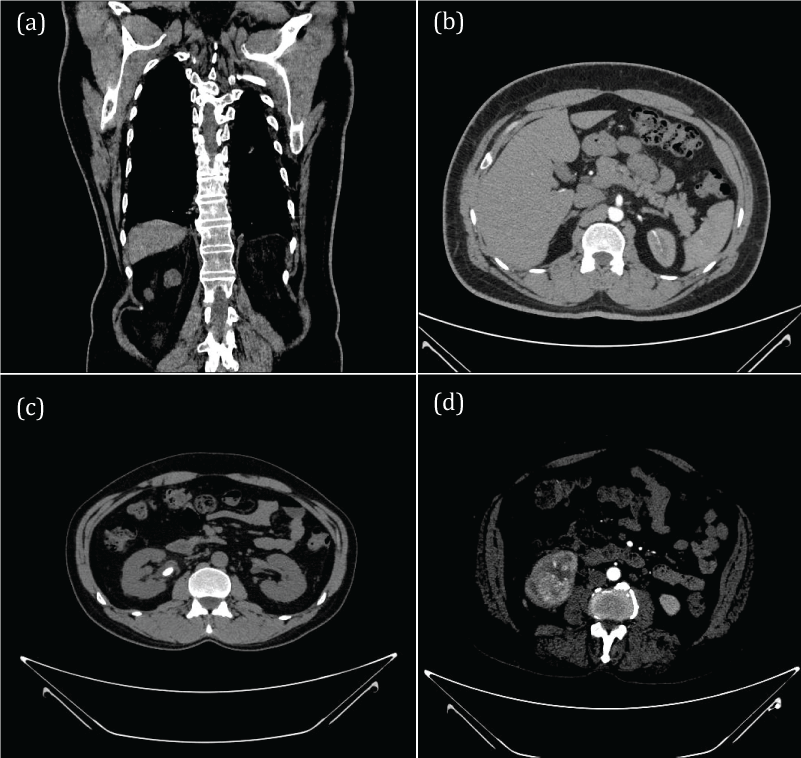
For kidney disease recognition, the dataset [26] was considered from “Islam, M. N., Hasan, M., Hossain, M. K., Alam, M. G. R., Uddin, M. Z., & Soylu, A. (2022). CT kidney dataset: Normal-cyst-tumor and stone [Data set].Kaggle. https://www.kaggle.com/datasets/nazmul0087/ct-kidney-dataset-normal-cyst-tumor-and-stone” repository which consists of four classes of images namely cyst, normal, stone, and tumor. The dataset was obtained from the Picture Archiving and Communication System (PACS) of several hospitals in Dhaka, Bangladesh, encompassing patients previously diagnosed with kidney tumor, cyst, stone, or normal renal conditions [26]. Coronal and axial slices were collected from both contrast-enhanced and non-contrast computed tomography studies, acquired under whole-abdomen and urogram imaging protocols [26]. Each DICOM study was systematically reviewed and categorized based on confirmed diagnosis, and representative region-of-interest (ROI) images corresponding to each radiological finding were carefully extracted to construct structured image batches [26]. To ensure patient privacy, all personally identifiable information and embedded metadata were removed from the DICOM files. The anonymized images were subsequently converted into a lossless JPG format without compromising image quality [26]. Following conversion, every image and its diagnostic label underwent a secondary verification process conducted jointly by an expert radiologist and a certified medical technologist to reaffirm dataset accuracy and clinical reliability [26]. The dataset has been taken from the kaggle repository directly without any augmentation or resizing procedures. The class “cyst” consists of 3,709 images. The class “normal” consists of 5,077 images. The class “stone” consists of 1,377 images. The class “tumor” consists of 2,283 images. In total, the total number of images in the dataset is 12,446. The dataset was separated into three subsets: training, validation, and test subsets. The training set consists of 9,335 images belonging to four classes. Similarly, the validation set consists of 1,867 images belonging to four classes. Finally, the test set consists of 1,244 images belonging to four classes. The training set considers 75% of the total dataset. Similarly, the validation set considers 15% of the total dataset. Finally, the test set considers the 10% of the total dataset. For the implementation of the deep CNN, the size of cyst image was resized from 705 × 569 to 160 × 160. Similarly, the size of the normal, stone, and tumor images were resized from 512 × 512 to 160 × 160. Next, for the implementation of VGG19 neural network, the size of the cyst image was resized from 705 × 569 to 224 × 224. Similarly, the size of the normal, stone, and tumor images were resized from 512 × 512 to 224 × 224. Finally, for the implementation of ResNet-50 deep neural network, the size of the cyst image was resized from 705 × 569 to 224 × 224. Similarly, the size of the normal, stone, and tumor images were resized from 512 × 512 to 224 × 224. The deep CNN, VGG19 neural network, and ResNet-50 neural network models were trained for 50 epochs on the dataset using the Adam optimizer with a learning rate of 0.0003, and categorical cross-entropy was used as a loss function. The deep CNN, VGG19 neural network, and ResNet-50 models were implemented in a TensorFlow environment using Python programming. A sample of one of the images belonging to each of the classes, namely “cyst”, “normal”, “stone”, and “tumor,” is shown in Figure 3.

Figure 3 images used for kidney disease recognition task. (a) cyst (b) normal (c) stone (d) tumor.

Figure 3: Images used for the kidney disease recognition task. (a) cyst (b) normal (c) stone (d) tumor.

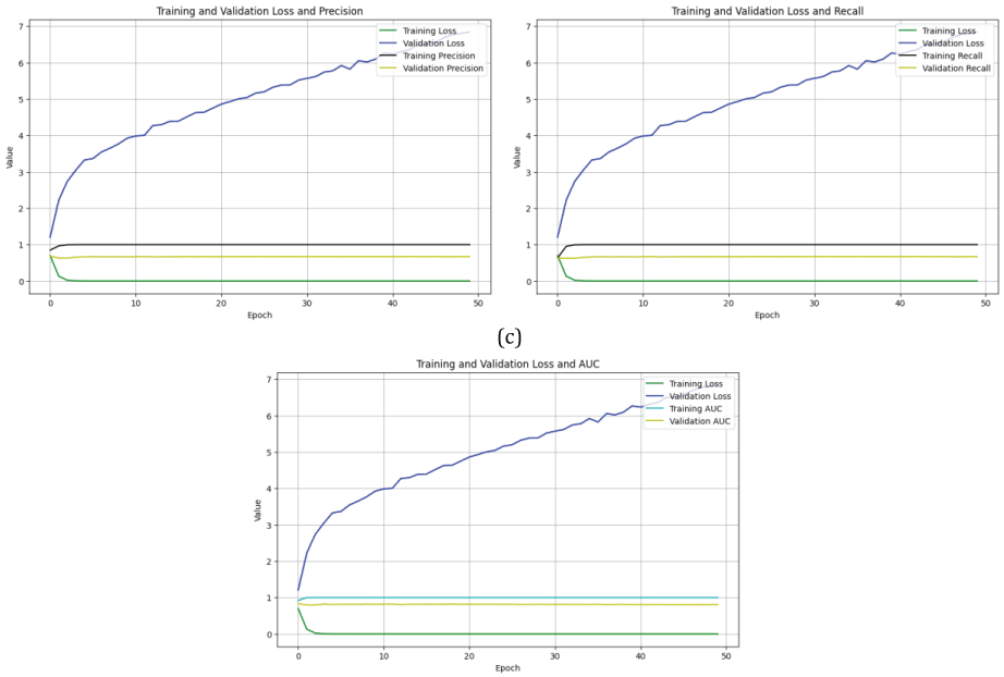
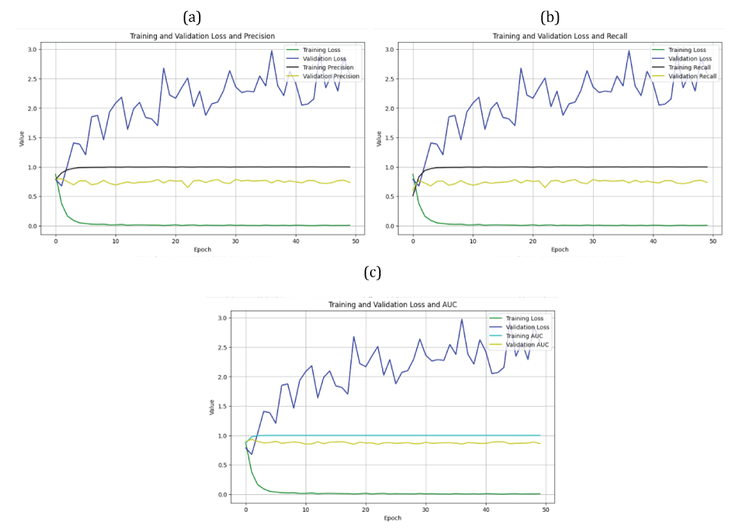
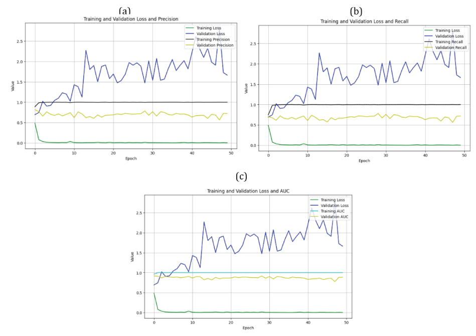
The deep CNN, VGG19 neural network, and ResNet-50 neural network models were trained on a subset of 24/28 images from the training/validation sets in a single epoch. Each epoch was iterated over 389/67 steps for the completion of the images on both sets. For training of deep CNN, VGG19 neural network, and ResNet-50 neural network models, the batch size considered was 24 images from the training set and 28 images from the validation set. The training of the deep CNN, VGG19 neural network, and ResNet-50 neural network models was done using a Graphics Processing Unit (GPU) Environment. The loss/PPV, loss/POD, and loss/AUC curves obtained from the deep CNN and VGG19 models are shown in Figure 4 and Figure 5.

Figure 4 (a-c) indicates that the margin between training error and validation error is higher; therefore, this indicates the deep CNN model is overfitting on the kidney disease image dataset [25, 27-35]. Further, Figure 4 (a-c) predicts that the margin between training PPV/POD/AUC and validation PPV/POD/AUC is also higher; therefore, the deep CNN model is not correctly fitting [25,27-35].

Figure 5 (a-c) also indicates that the margin between training error and validation error is higher; therefore, the VGG19 model is overfitting on the kidney disease image dataset [25, 27-35]. Further, Figure 5 (a-c) depicts that the margin between training PPV/POD/AUC and validation PPV/POD/AUC is also higher; therefore, the VGG19 model is not correctly fitting [25, 27-35].

Figure 4: loss/PPV, loss/POD, and loss/AUC curves obtained from the deep CNN model: (a) loss/positive-predictive-value (PPV) curve from deep CNN (b) loss/probability of detection (POD) curve from deep CNN (c) loss/Area under Curve (AUC) curve from deep CNN.

Figure 5: loss/PPV, loss/POD, and loss/AUC curves obtained from the VGG19 model: (a) loss/PPV curve from the VGG19 model, (b) loss/POD curve from the VGG19 model, (c) loss/AUC curve from the VGG19 model.

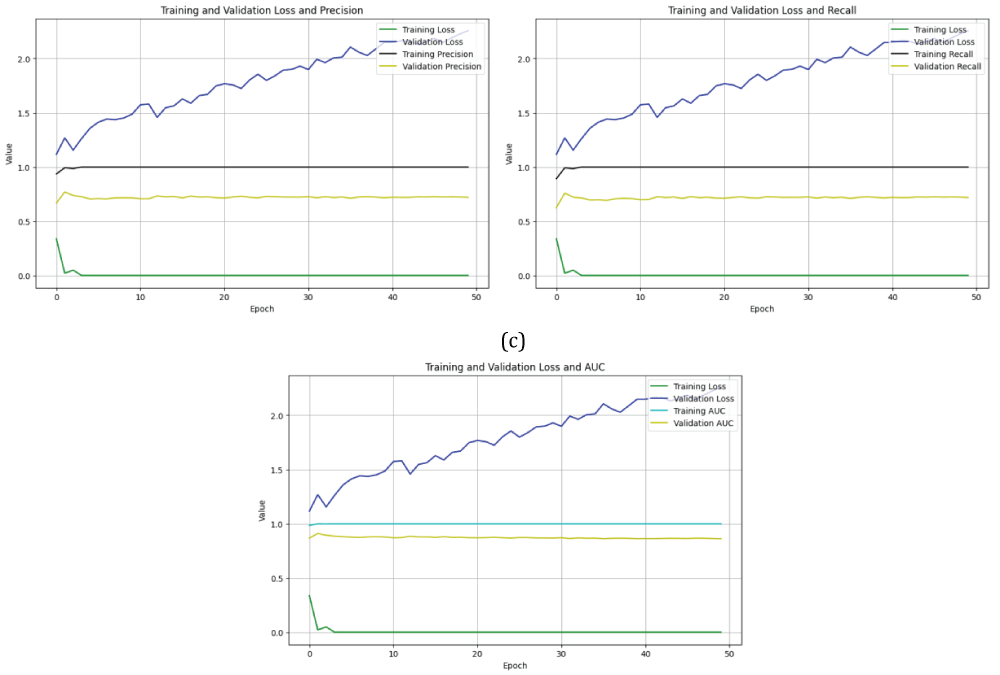
After applying a dropout of 0.5 on both the deep CNN and VGG19 neural network models, the loss/PPV, loss/POD, and loss/AUC curves obtained from the deep CNN and VGG19 models are shown in Figure 6 and Figure 7.

Figure 6: loss/PPV, loss/POD, and loss/AUC curves obtained from the deep CNN model after applying the dropout regularization technique: (a) loss/PPV curve from the deep CNN, (b) loss/POD curve from the deep CNN, (c) loss/AUC curve from the deep CNN.

Figure 7: loss/PPV, loss/POD, and loss/AUC curves obtained from the VGG19 model after applying the dropout regularization technique: (a) loss/PPV curve from the VGG19 model, (b) loss/POD curve from the VGG19 model, (c) loss/AUC curve from the VGG19 model.

After applying a dropout of 0.5, Figure 6 (a-c) shows that the margin between training error and validation error is a little bit reduced compared to Figure 4 (a-c), i.e the validation error is reduced compared to the previous case before applying the dropout condition. Therefore, this indicates the deep CNN is still overfitting on the kidney disease image dataset even after applying the dropout regularization technique. Further,

Figure 6 (a-c) depicts that the margin between training PPV/POD/AUC and validation PPV/POD/AUC is also higher; therefore, this indicates the deep CNN model is still not correctly fitting [25,27-35].

After applying a dropout of 0.5, Figure 7 (a-c) depicts that the margin between training error and validation error is a little bit reduced compared to Figure 5 (a-c), i.e the validation error is reduced compared to the previous case before applying the dropout condition; therefore, this indicates the VGG19 model is over fitting on kidney disease image dataset even after applying drop out regularization technique. Further, Figure 7 (a-c) indicates the margin between training PPV/POD/AUC and validation PPV/POD/AUC is also higher; therefore, this indicates the VGG19 model is not correctly fitting [25, 27-35]. In this manner, it can now be depicted that even after applying the dropout regularization technique, the CNN and VGG19 models are still not correctly fitting the kidney disease image dataset.

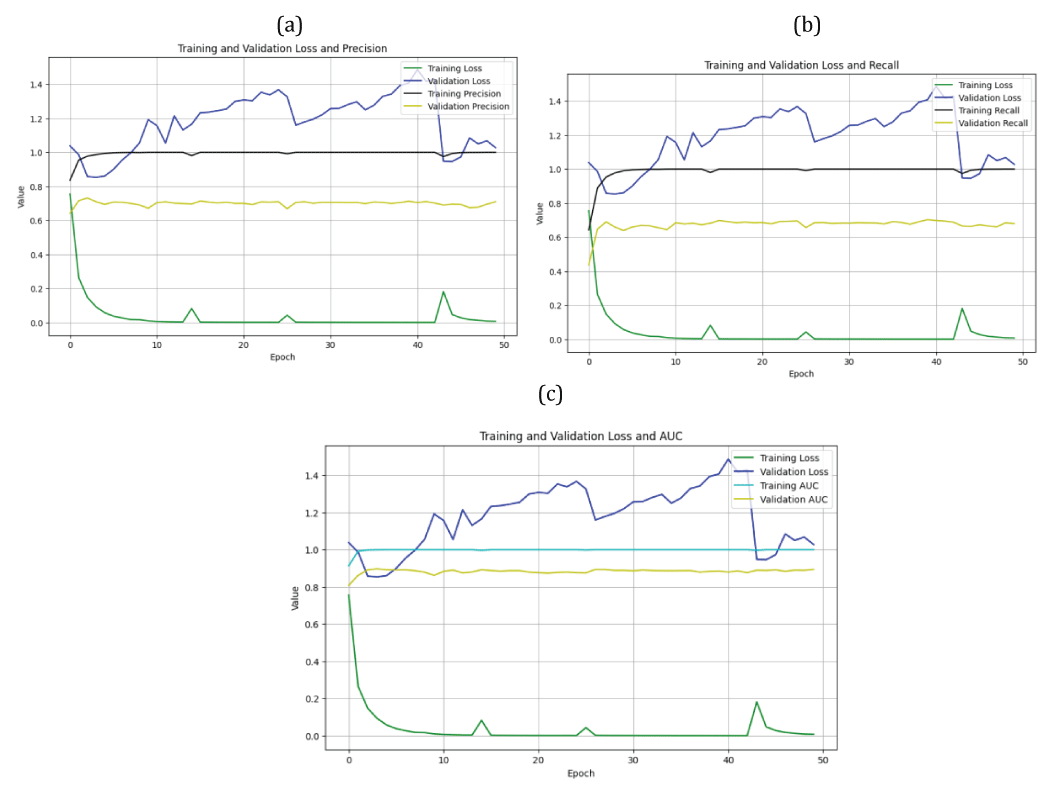
The loss/PPV, loss/POD, and loss/AUC curves obtained from the deep residual network, i.e., the ResNet-50 neural network, are shown in Figure 8.

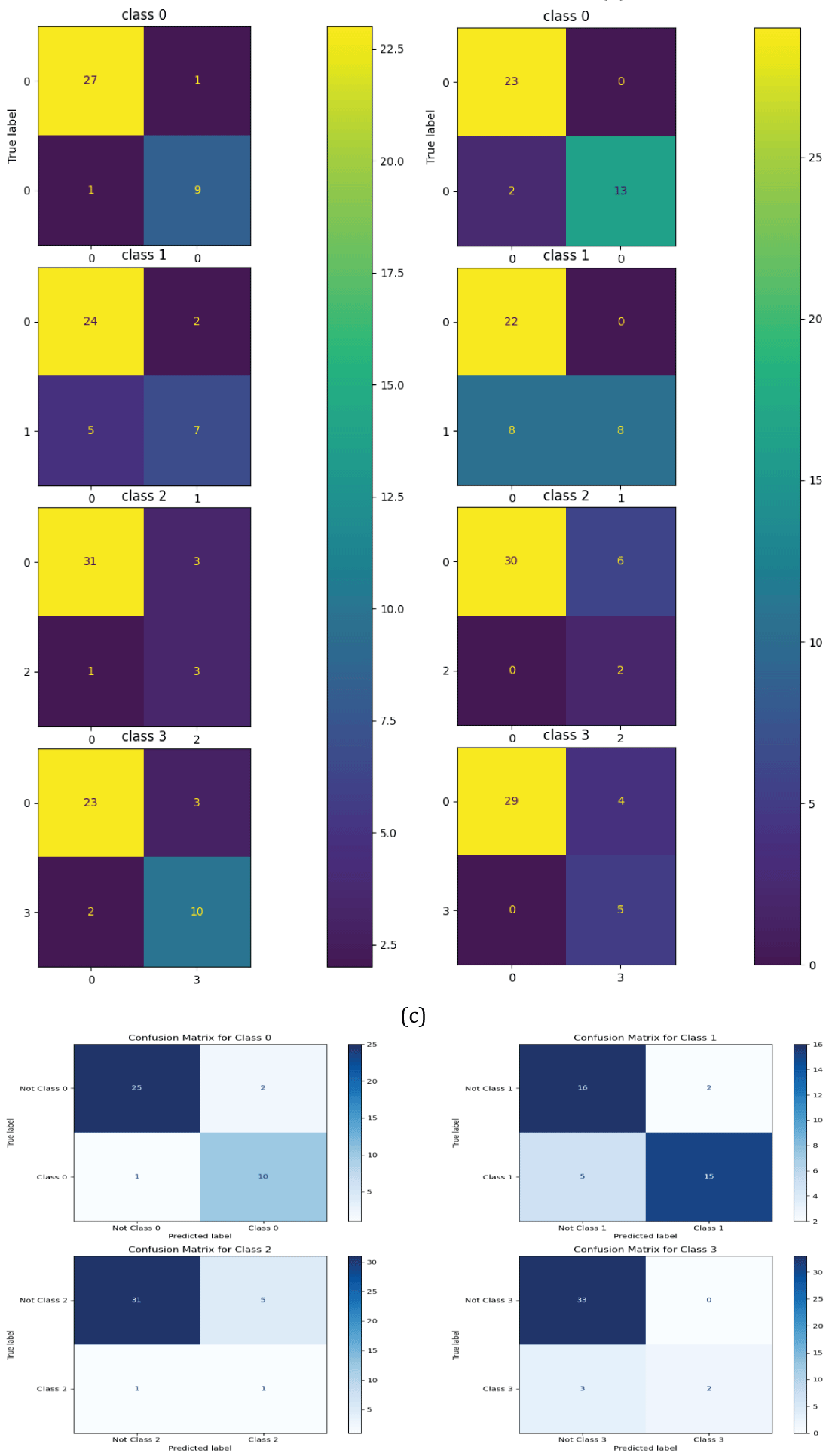
Figure 8 (a-c) also indicates that the margin between training error and validation error is lower; therefore, the deep residual network, i.e., the ResNet-50 model, is correctly fitting the kidney disease image dataset [25, 27-35]. Further, Figure 8 (a-c) depicts that the margin between training PPV/POD/AUC and validation PPV/POD/AUC is also lower; therefore, the ResNet-50 model is correctly fitting [25, 27-35]. The deep CNN, VGG19 neural network, and ResNet-50 neural network models were tested on a batch of 38 images from the test dataset. The confusion matrix obtained from the deep CNN, VGG19 neural network, and ResNet-50 neural network models is shown in Figure 9 [25,27-35].

Figure 8: loss/PPV, loss/POD, and loss/AUC curves obtained from the deep residual network model (ResNet-50): (a) loss/PPV curve from the ResNet-50 model, (b) loss/POD curve from the ResNet-50 model, (c) loss/AUC curve from the ResNet-50 model.

The confusion matrix obtained from the deep CNN model is shown in Figure 9 (a) for all four classes [25,27-35].

For class cyst, 28 images are recognised as belonging to not cyst and 10 images are recognised as cyst. Further from Figure 9 (a), 27 (TN) images which are actually not cyst have been recognised as not cyst, 9 (TP) images which are actually cyst are predicted as cyst, 1 (FP) image which is actually not cyst has been predicted as cyst, and finally 1 (FN) image which is actually cyst has been predicted as non-cyst.

For the class normal, 26 images are recognised as not normal and 12 images are recognised as belonging to normal. From Figure 9 (a), 24 (TN) images which are actually not normal have been predicted as not normal, 2 (FP) images which are not normal have been predicted as normal, 5 (FN) images which are normal have been predicted as not normal, and finally 7 (TP) images which are normal have been predicted as normal.

For the class stone, 34 images are recognised as not stone and 4 images are recognised as belonging to stone. From Figure 9 (a), 31 (TN) images which are actually not stone have been predicted as not stone, 3 (FP) images which are not stone have been predicted as stone, 1 (FN) image which is stone has been predicted as not stone, and finally 3 (TP) images which are stone have been predicted as stone.

For the class tumor, 26 images are recognised as not tumor and 12 images are recognised as belonging to tumor. From Figure 9 (a), 23 (TN) images which are actually not tumor have been predicted as not tumor, 3 (FP) images which are not tumor have been predicted as tumor, 2 (FN) images which are tumor have been predicted as not tumor, and finally 10 (TP) images which are tumor have been predicted as tumor.

Figure 9: Confusion matrix from deep CNN, VGG19, and ResNet-50 neural network models: (a) deep CNN, (b) VGG19 model, (c) ResNet-50 model

The confusion matrix obtained from the VGG19 model is shown in Figure 9 (b) for all four classes [25,27-35].

For the class cyst, 23 images are recognised as belonging to not cyst and 15 images are recognised as cyst. Further from Figure 9 (b), 23 (TN) images which are actually not cyst have been recognised as not cyst, 13 (TP) images which are actually cyst are predicted as cyst, 0 (FP) images which are actually not cyst have been predicted as cyst, and finally 2 (FN) images which are actually cyst have been predicted as non-cyst.

For the class normal, 22 images are recognised as not normal and 16 images are recognised as belonging to normal. From Figure 9 (b), 22 (TN) images which are actually not normal have been predicted as not normal, 0 (FP) images which are not normal have been predicted as normal, 8 (FN) images which are normal have been predicted as not normal, and finally 8 (TP) images which are normal have been predicted as normal.

For the class stone, 36 images are recognised as not stone and 2 images are recognised as belonging to stone. From Figure 9 (b), 30 (TN) images which are actually not stone have been predicted as not stone, 6 (FP) images which are not stone have been predicted as stone, 0 (FN) images which are stone have been predicted as not stone, and finally 2 (TP) images which are stone have been predicted as stone.

For the class tumor, 33 images are recognised as not tumor and 5 images are recognised as belonging to tumor. From Figure 9 (b), 29 (TN) images that are actually not tumor have been predicted as not tumor, 4 (FP) images which are not tumor have been predicted as tumor, 0 (FN) images which are tumor have been predicted as not tumor, and finally 5 (TP) images which are tumor have been predicted as tumor.

The confusion matrix obtained from the ResNet-50 model is shown in Figure 9 (c) for all four classes [25,27-35].

For class cyst, 27 images are recognised as belonging to not cyst and 11 images are recognised as cyst. Further from Figure 9 (c), 25 (TN) images that are actually not cyst have been recognised as not cyst, 10 (TP) images which are actually cyst are predicted as cyst, 2 (FP) images which are actually not cyst have been predicted as cyst, and finally 1 (FN) image which is actually cyst has been predicted as non-cyst.

For the class normal, 18 images are recognised as not normal and 20 images are recognised as belonging to normal. From Figure 9 (c), 16 (TN) images which are actually not normal have been predicted as not normal, 2 (FP) images which are not normal have been predicted as normal, 5 (FN) images which are normal have been predicted as not normal, and finally 15 (TP) images which are normal have been predicted as normal.

For the class stone, 36 images are recognised as not stone and 2 images are recognised as belonging to stone. From Figure 9 (c), 31 (TN) images which are actually not stone have been predicted as not stone, 5 (FP) images which are not stone have been predicted as stone, 1 (FN) image which is stone has been predicted as not stone, and finally 1 (TP) image which is stone has been predicted as stone.

For the class tumor, 33 images are recognised as not tumor and 5 images are recognised as belonging to tumor. From Figure 9 (c), 33 (TN) images which are actually not tumor have been predicted as not tumor, 0 (FP) images which are not tumor have been predicted as tumor, 3 (FN) images which are tumor have been predicted as not tumor, and finally 2 (TP) images which are tumor have been predicted as tumor.

The performance metrics such as accuracy, PPV, POD, and F1-score values obtained from deep CNN, VGG19 neural network, and ResNet-50 neural network models are shown in Tables 4, 5, and 6.

The performance metrics such as accuracy, PPV, POD, and F1-score values obtained from the deep CNN model for all four classes, namely cyst, normal, stone, and tumor, are shown in Table 4. The performance metrics such as accuracy, PPV, POD, and F1-score are calculated from the confusion matrix. The metric accuracy is defined as the ratio of true predictions to the sum of all predictions. The mathematical equation for accuracy is shown in Eqn. (1).

$Accuracy=\frac{True Positive \left(TP\right)+True Negative (TN)}{True Positive \left(TP\right)+True Negative \left(TN\right)+False Positive \left(FP\right)+False Negative (FN)}$ (1)

The metric PPV is defined as the ratio of label TP to the sum of labels TP and FP. The metric PPV is also called precision. The mathematical equation for precision is shown in Eqn. (2).

$precision=\frac{TP}{TP+FP}$ (2)

The metric POD is defined as the ratio of label TP to the sum of labels TP and FN. The metric POD is also called recall. The mathematical equation for recall is shown in Eqn. (3).

$Recall=\frac{TP}{TP+FN}$ (3)

The metric F1-score is defined as the harmonic mean of PPV and POD metrics. The mathematical equation for F1-score is shown in Eqn. (4).

$F1-Score=\frac{2*precision*recall}{precision+recall}$ (4)

The overall accuracy for class cyst obtained from the deep CNN model is 0.95. The deep CNN has PPV of 0.90/POD of 0.90/F1-score of 0.90 for class cyst. The overall accuracy for class normal obtained from the deep CNN model is 0.82. The deep CNN has PPV of 0.78/POD of 0.58/F1-score of 0.67 for class normal. The overall accuracy for class stone obtained from the deep CNN model is 0.89. The deep CNN has PPV of 0.50/POD of 0.75/F1-score of 0.60 for class stone. The overall accuracy for class tumor obtained from the deep CNN model is 0.87. The deep CNN has PPV of 0.77/POD of 0.83/F1-score of 0.80 for class tumor.

The overall accuracy obtained from the deep CNN model reported is higher for class cyst compared to the normal, stone, and tumor categories on the test set. The class normal has lower accuracy compared to the other three classes, i.e cyst, stone, and tumor categories.

The classification report obtained from the VGG19 neural network for all four classes, namely cyst, normal, stone, and tumor, is shown in Table 5. The overall accuracy for class cyst obtained from the VGG19 neural network is 0.95. The VGG19 neural network has PPV of 1.00/POD of 0.87/F1-score of 0.93 for class cyst. The overall accuracy for class normal obtained from the VGG19 neural network is 0.79. The VGG19 neural network has PPV of 1.00/POD of 0.50/F1-score of 0.67 for class normal. The overall accuracy for class stone obtained from the VGG19 neural network is 0.84. The VGG19 neural network has PPV of 0.25/POD of 1.00/F1-score of 0.40 for class stone. The overall accuracy for class tumor obtained from the VGG19 neural network is 0.89. The VGG19 neural network has a PPV of 0.56/POD of 1.00/F1-score of 0.71 for class tumor.

The overall accuracy obtained from the VGG19 model reported is higher for class cyst compared to the normal, stone, and tumor categories on the test set. The class normal has lower accuracy compared to the other three classes, i.e cyst, stone, and tumor categories.

The overall accuracy for class cyst obtained from the ResNet-50 model is 0.92. The ResNet-50 model has a PPV of 0.83/POD of 0.90/F1-score of 0.86 for class cyst. The overall accuracy for class normal obtained from the ResNet-50 model is 0.82. The ResNet-50 model has a PPV of 0.88/POD of 0.75/F1-score of 0.81 for class normal. The overall accuracy for class stone obtained from the ResNet-50 model is 0.84. The ResNet-50 model has PPV of 0.17/POD of 0.50/F1-score of 0.25 for class stone. The overall accuracy for class tumor obtained from the ResNet-50 model is 0.92. The ResNet-50 model has a PPV of 1.00/POD of 0.40/F1-score of 0.51 for class tumor. The overall accuracy obtained from the ResNet-50 model reported is higher for class cyst compared to the normal, stone, and tumor categories on the test set. The class normal has lower accuracy compared to the other three classes, i.e cyst, stone, and tumor categories.

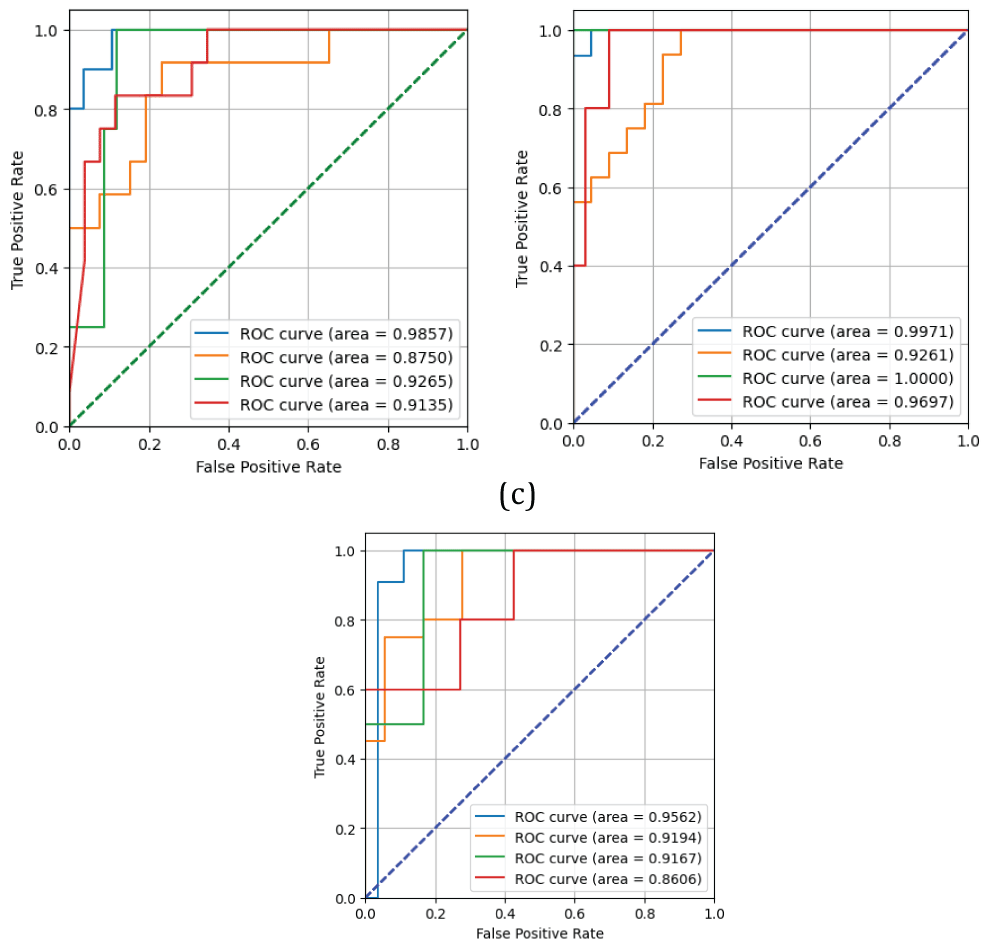
The specificity/POD curves obtained from both the deep CNN and VGG19 models are shown in Figure 10 [25,27-35]. The specificity/POD curve, i.e., the Receiver Operating Characteristic (ROC) curve, is mainly used for binary/multi-class classification tasks. The Area under Curve (AUC) is used as one of the measures in the ROC. The AUC curve is plotted by considering false positive rate (FPR) along the x-axis and true positive rate (TPR) along the y-axis. The AUC value of 1.00 indicates the performance of the classifier is excellent. The AUC value in the ROC curve is obtained by considering the relationship between true labels and score values obtained from the true features of the test set. Figure 10 (a) depicts that the deep CNN model has an AUC value of 0.98 for class “cyst”, 0.87 for class “normal”, 0.92 for class “stone”, and 0.91 for class “tumor” [25,27-35]. The deep CNN model has the highest AUC value for class “cyst” compared to other classes. Next, Figure 10 (b) depicts that the VGG19 model has an AUC value of 0.99 for class “cyst”, 0.92 for class “normal”, 1.00 for class “stone”, and 0.96 for class “tumor” [25,27-35]. The VGG19 model has the highest AUC value for class “stone” compared to other classes.

Finally, Figure 10 (c) depicts that the ResNet-50 model has an AUC value of 0.96 for class “cyst”, 0.92 for class “normal”, 0.92 for class “stone”, and 0.86 for class “tumor” [25,27-35]. The ResNet-50 model has the highest AUC value for class “cyst” compared to the other classes.

Figure 10: Specificity/POD curve from the deep CNN, VGG19, and ResNet-50 models (a) deep CNN (b) VGG19 (c) ResNet-50.

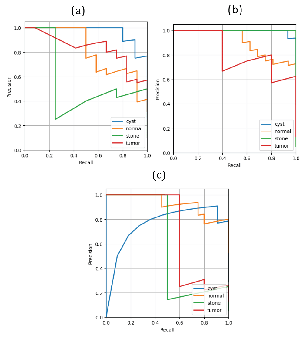
The PPV/POD curves obtained from the deep CNN, VGG19, and ResNet-50 models are shown in Figure 11 [25,27-35].

Figure 11: PPV/POD curves from deep CNN, VGG19, and ResNet-50 models (a) deep CNN (b) VGG19 model (c) ResNet-50 model.

The PPV/POD curve, i.e., the precision/recall characteristic, is also used to measure the performance of binary/multi-class classifiers. Figure 11 (a) depicts that the deep CNN has a PPV of 0.90 as POD approaches 0.90 for class “cyst”, 0.78 of PPV as POD approaches 0.58 for class “normal”, 0.50 of PPV as POD approaches 0.75 for class “stone”, and 0.77 of PPV as POD approaches 0.83 for class “tumor” [25,27-35]. The deep CNN has the highest PPV as POD approaches lower for class “normal”. The deep CNN has lower PPV as POD approaches higher for classes “stone” and “tumor”. The deep CNN has equal values of PPV and POD for class “cyst”.

Figure 11 (b) indicates the VGG19 model has a PPV of 1.00 as POD approaches 0.97 for class “cyst”, a PPV of 1.00 as POD approaches 0.50 for class “normal”, 0.25 of PPV as POD approaches 1.00 for class “stone”, and 0.56 of PPV as POD approaches 1.00 for class “tumor”. The VGG19 model has the highest PPV as POD approaches lower for classes “cyst” and “normal” [25,27-35]. The VGG19 model has lower PPV as POD approaches higher for classes “stone” and “tumor”.

Figure 11 (c) indicates the ResNet-50 model has a PPV of 0.83 as POD approaches 0.90 for class “cyst”, a PPV of 0.88 as POD approaches 0.75 for class “normal”, 0.17 of PPV as POD approaches 0.50 for class “stone”, and a PPV of 1.00 as POD approaches 0.40 for class “tumor”. The ResNet-50 model has the highest PPV as POD approaches lower values for classes “normal” and “tumor” [25,27-35]. The ResNet-50 model has lower PPV as POD approaches higher for classes “cyst” and “stone”.

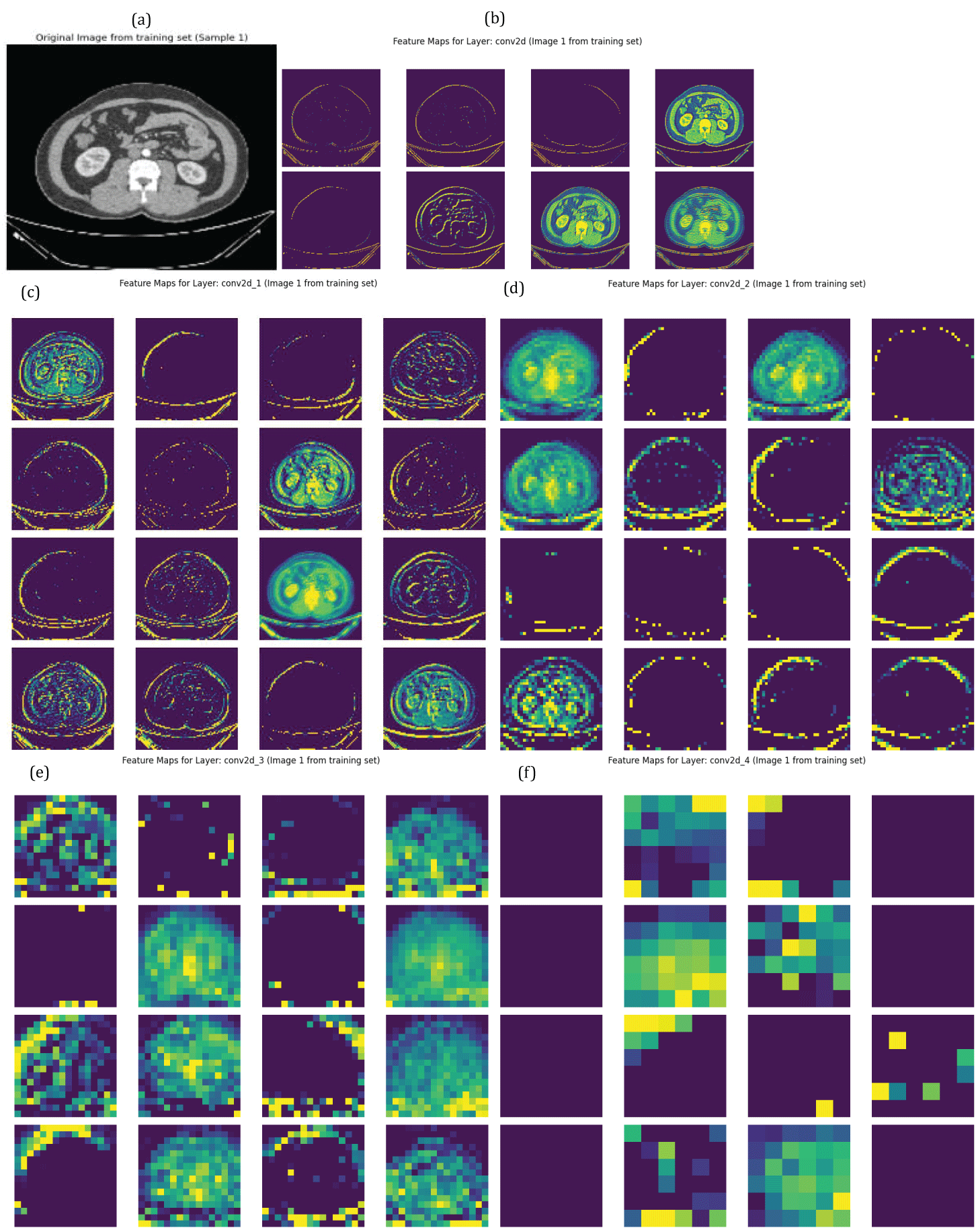
The feature maps obtained from the five convolutional layers on a sample of a single training image are shown in Figure 12.

Figure 12: Feature Maps of Five Convolutional Layers obtained from deep CNN model (a) original image (b) convolutional layer1 output (c) convolutional layer2 output (d) convolutional layer3 output (e) convolutional layer4 output (f) convolutional layer5 output.

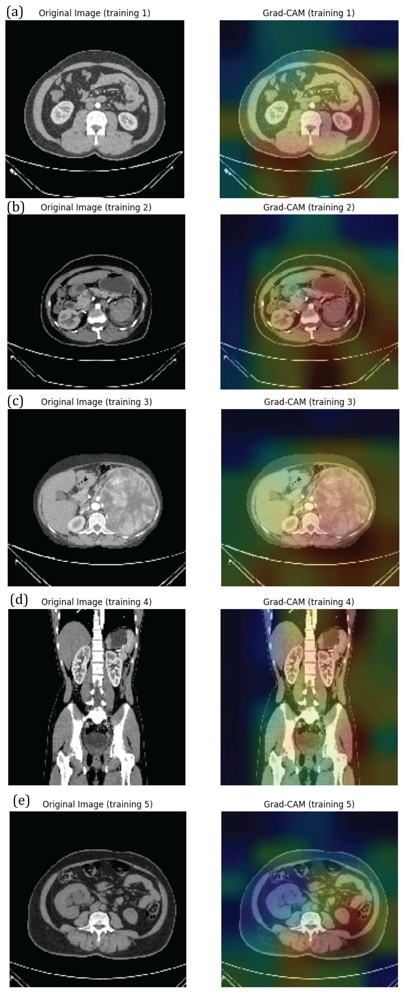
The Grad-CAM output obtained from the deep CNN model on a sample of five training images is shown in Figure 13.

Figure 13: Grad-Cam Visualizations obtained from deep CNN model (a) Training image1 (b) Training image2 (c) Training image3 (d) Training image4 (e) Training image5.

Conclusion

In this paper, computed tomography kidney disease recognition has been performed using various deep neural networks such as deep CNN, visual geometry group (VGG)-19 layer neural network, and deep residual network, i.e ResNet-50 neural network. Kidney disease recognition has been performed on the dataset, which consists of four classes of images, namely “cyst”, “normal”, “stone”, and “tumor”. The deep CNN, VGG-19, and ResNet-50 layer neural network models were trained on the dataset to produce the results. The results, such as loss/PPV/POD/AUC curves on training/validation sets, confusion matrix, specificity/POD curve, and PPV/POD curves, are shown for the confirmation of the work [25,27-35]. From the loss/PPV/POD/AUC curves, it can be depicted that the deep CNN and VGG19 models are overfitting on the kidney disease image dataset [25,27-35]. Further, a dropout of 0.5 is applied to both the deep CNN and VGG19 neural network models to mitigate the overfitting issue. Further, from the loss/PPV/POD/AUC curves of the ResNet-50 model, it can be depicted that the ResNet-50 model is correctly fitting on the kidney disease image dataset [25,27-35]. The feature maps and Grad-CAM visualizations for a sample of a single training image/five training images obtained from the deep CNN model are also shown in the work. Next, from the confusion matrix, it can be predicted that the deep CNN and VGG19 models have a higher number of images for the FALSE label compared to the TRUE label for each of the four classes, respectively [25,27-35]. Further, from the confusion matrix, it can be predicted that the ResNet-50 neural network model has a higher number of images for the FALSE label compared to the TRUE label for all three classes, such as cyst, stone, and tumor classes, except the normal class [25,27-35]. Next, from the specificity/POD curve, it can be observed that the deep CNN, VGG19, and ResNet-50 neural network models have higher AUC values for all four classes, respectively. The deep CNN has the highest AUC value for class “cyst” compared to the other three classes. The VGG19 layer neural network has a perfect AUC value of 1.00 for class “stone” compared to the remaining three classes [25,27-35]. The ResNet-50 model has the highest AUC value for class “cyst” compared to the other classes. Finally, it can be said that the VGG19 layer neural network has higher AUC values for all four classes compared to the deep CNN and ResNet-50 neural network models [25, 27-35]. Therefore, it can be concluded that the VGG19 neural network has better kidney disease recognition performance compared to deep CNN and deep residual neural network models.

Limitations and future scope

The present paper demonstrates computed tomography kidney disease recognition using deep neural networks such as deep CNN, VGG19 neural network, and ResNet-50 neural network models. These deep neural networks have been trained on the kidney disease dataset to produce the results. From loss/PPV, loss/POD, and loss/AUC curves, it can be said that the deep CNN and VGG19 neural network models are overfitting on the kidney disease dataset. To overcome overfitting, a regularization technique such as dropout was applied to overcome this issue. But still, after applying a dropout of 0.5, overfitting was not reduced. So, to further mitigate this overfitting issue, pre-trained models such as the deep residual network, i.e., the ResNet-50 model, were applied. To further mitigate the overfitting issue, several other pre-trained neural network models such as DenseNet and Neural Architecture Search (NAS) neural networks can be applied. Next, another major drawback of this research work is single computed tomography kidney disease dataset has been considered in this research work. So these deep neural networks, such as deep CNN, VGG19, and ResNet-50 models, can be applied to external clinical imaging datasets from other repositories or from other modalities for the kidney disease recognition task. Further, in the future, these deep learning neural networks can be applied for holographic live cell imaging of computed tomography kidney disease images to perform a binary/multi-class classification task. These deep neural network models can also be used for binary classification of normal versus cyst/stone/tumor images in future work. Finally, these deep neural networks can be applied for brain-tumor recognition and heart-attack-analysis prediction tasks.

References

1. Farooq MS, Tariq A. A deep learning architectures for kidney disease classification. arXiv. 2024. doi:10.48550/arXiv.2403.15895

2. Mohsen S, Ali AM, El-Rabaie ESM, ElKaseer A, Scholz SG, Hassan AMA. Brain tumor classification using hybrid single image super-resolution technique with ResNeXt101_32×8d and VGG19 pre-trained models. IEEE Access. 2023;11:55582–55595. doi:10.1109/ACCESS.2023.3281529

3. Hossain MI, Maruf MH, Khan MAR, Prity FS, Fatema S, Ejaz MS, Khan MAS. Heart disease prediction using distinct artificial intelligence techniques: Performance analysis and comparison. Iran J Comput Sci. 2023;6(4):397–417. doi:10.1007/s42044-023-00148-7

4. Jacobson SH. Chronic kidney disease—A public health problem? Lakartidningen. 2013;110(21):1018–1020.

5. Jha V, Garcia-Garcia G, Iseki K, Li Z, Naicker S, Plattner B, Remuzzi G, Yang CW. Chronic kidney disease: Global dimension and perspectives. Lancet. 2013;382(9888):260–272. doi:10.1016/S0140-6736(13)60687-X

6. Foreman KJ, Marquez N, Dolgert A, Fukutaki K, Fullman N, McGaughey M, Pletcher MA, Smith AE, Tang K, Yuan CW, Brown JC, Friedman J, He J, Heuton KR, Holmberg M, Patel DJ, Reidy P, Carter A, Cercy K, Murray CJL. Forecasting life expectancy, years of life lost, and all-cause and cause-specific mortality for 250 causes of death: Reference and alternative scenarios for 2016–40 for 195 countries and territories. Lancet. 2018;392(10159):2052–2090. doi:10.1016/S0140-6736(18)31694-5

7. Rediger C, Guerra LA, Keays MA, Wayne C, Reddy D, Ksara S, Leonard MP. Renal cyst evolution in childhood: A contemporary observational study. J Pediatr Urol. 2019;15(2):188.e1–188.e7. doi:10.1016/j.jpurol.2018.12.012

8. Brownstein AJ, Bin Mahmood SU, Saeyeldin A, Velasquez Mejia C, Zafar MA, Li Y, Ziganshin BA, Rizzo JA, Elefteriades JA. Simple renal cysts and bovine aortic arch: Markers for aortic disease. Open Heart. 2019;6(1):e000862. doi:10.1136/openhrt-2018-000862

9. Sanna E, Loukogeorgakis S, Prior T, Derwig I, Paramasivam G, Choudhry M, Lees C. Fetal abdominal cysts: Antenatal course and postnatal outcomes. J Perinat Med. 2019;47(4):418–421. doi:10.1515/jpm-2018-0319

10. Alelign T, Petros B. Kidney stone disease: An update on current concepts. Adv Urol. 2018;2018:3068365. doi:10.1155/2018/3068365

11. Hsieh JJ, Purdue MP, Signoretti S, Swanton C, Albiges L, Schmidinger M, Heng DYC, Larkin J, Ficarra V, Renal Cell Carcinoma Working Group. Renal cell carcinoma. Nat Rev Dis Primers. 2017;3(1):17009. doi:10.1038/nrdp.2017.9

12. Sozio SM, Pivert KA, Caskey FJ, Levin A. The state of the global nephrology workforce: A joint ASN–ERA-EDTA–ISN investigation. Kidney Int. 2021;100(5):995–1000. doi:10.1016/j.kint.2021.08.011

13. Wasi S, Alam SB, Rahman R, Amin MA, Kobashi S. Kidney tumor recognition from abdominal CT images using transfer learning. In: 2023 IEEE 53rd International Symposium on Multiple-Valued Logic (ISMVL). IEEE; 2023. p.54–58. doi:10.1109/ISMVL57333.2023.00021

14. Prommakhot A, Srinonchat J. VGGNet integration for kidney tumor classification. In: 2024 12th International Electrical Engineering Congress (iEECON). IEEE; 2024. p.1–6. doi:10.1109/iEECON60677.2024.10537904

15. Brehar RD, Mitrea DA, Nedevschi S, Moisoiu T, Elec FI, Socaciu MA. Kidney tumor segmentation and grade identification in CT images. In: 2023 IEEE 19th International Conference on Intelligent Computer Communication and Processing (ICCP). IEEE; 2023. p.293–300. doi:10.1109/ICCP60212.2023.10398718

16. Yang G, Li G, Pan T, Kong Y, Wu J, Shu H, Zhu X. Automatic segmentation of kidney and renal tumor in CT images based on 3D fully convolutional neural network with pyramid pooling module. In: 2018 24th International Conference on Pattern Recognition (ICPR). IEEE; 2018. p.3790–3795. doi:10.1109/ICPR.2018.8545143

17. Zhao Z, Chen H, Li J, Wang L. Boundary attention u-net for kidney and kidney tumor segmentation. In: 2022 44th Annual International Conference of the IEEE Engineering in Medicine & Biology Society (EMBC). IEEE; 2022. p.1540–1543. doi:10.1109/EMBC48229.2022.9871443

18. Islam MN, Hasan M, Hossain MK, Alam MGR, Uddin MZ, Soylu A. Vision transformer and explainable transfer learning models for auto detection of kidney cyst, stone and tumor from CT-radiography. Sci Rep. 2022;12(1):11440. doi:10.1038/s41598-022-15634-4

19. Alzu’bi D, Abdullah M, Hmeidi I, AlAzab R, Gharaibeh M, El-Heis M, Abualigah L. Kidney tumor detection and classification based on deep learning approaches: A new dataset in CT scans. J Healthc Eng. 2022;2022(1):3861161. doi:10.1155/2022/3861161

20. Hossain MN, Bhuiyan E, Miah MBA, Sifat TA, Muhammad Z, Masud MFA. Detection and classification of kidney disease from CT images: An automated deep learning approach. Technologies. 2025;13(11):508. doi:10.3390/technologies13110508

21. Jahan F, Reza AS, Morol MK, Nandi D, Hossen MJ, Rahman M. Explainable deep learning for early diagnosis of chronic kidney disease from CT images in Bangladeshi patients. Sci Rep. 2026;16(1):14819. doi:10.1038/s41598-026-42654-1

22. Kumar Y, Brar TPS, Kaur C, Singh C. A comprehensive study of deep learning methods for kidney tumor, cyst, and stone diagnostics and detection using CT images. Arch Comput Methods Eng. 2024;31(7):4163–4188. doi:10.1007/s11831-024-10112-8

23. Vemula N, Nandan D. Kidney Disease Detection Using Computed Tomography Scans: A Deep Learning Approach with Hybrid Activation Functions Based ResNet50. In: 2025 IEEE International Conference on Advanced Computing Technologies (ICACT). IEEE; 2025. p.701–706.

24. He K, Zhang X, Ren S, Sun J. Deep residual learning for image recognition. In: Proceedings of the IEEE Conference on Computer Vision and Pattern Recognition. IEEE; 2016. p.770–778. doi:10.1109/CVPR.2016.90

25. Mahesh RN U, Nelleri A. Multi-class classification and multi-output regression of three-dimensional objects using artificial intelligence applied to digital holographic information. Sensors. 2023;23(3):1095. doi:10.3390/s23031095

26. Islam MN, Hasan M, Hossain MK, Alam MGR, Uddin MZ, Soylu A. CT kidney dataset: Normal-cyst-tumor and stone [Data set]. Kaggle. 2022. Available from: https://www.kaggle.com/datasets/nazmul0087/ct-kidney-dataset-normal-cyst-tumor-and-stone

27. Reddy BL, Uma Mahesh RN, Nelleri A. Deep convolutional neural network for three-dimensional objects classification using off-axis digital Fresnel holography. J Mod Opt. 2022;69(13):705–717. doi:10.1080/09500340.2022.2081371

28. Uma Mahesh RN, Lokesh Reddy B, Nelleri A. Deep learning-based multi-class 3D objects classification using digital holographic complex images. In: International Conference on Futuristic Communication and Network Technologies. Singapore: Springer Nature Singapore; 2020. p.443–448. doi:10.1007/978-981-16-4625-6_43

29. Mahesh U, Kiran B. Three-dimensional (3-D) objects classification by means of phase-only digital holographic information using Alex Network. In: 2024 International Conference on Signal Processing, Computation, Electronics, Power and Telecommunication (IConSCEPT). IEEE; 2024. p.1–5. doi:10.1109/IConSCEPT61884.2024.10627906

30. Mahesh U, HJ HJ, Kumar H, Umrao S, DL M. Melanocytic Nevi Classification using Transfer Learning. Igmin Res. 2025;3(7):258–267. doi:10.61927/igmin307

31. Mahesh RU, Nagaraju S. Three-dimensional (3-D) objects classification by means of phase-only digital holographic information using deep learning. In: Data science & exploration in artificial intelligence. A.A. Balkema; 2025. p.363–371. doi:10.1201/9781003587392-53

32. Mahesh U, Madhusudhan KV. Clustering of Three-dimensional (3-D) Objects by Means of Phase-only Digital Holographic Information using Machine Learning. Igmin Res. 2025;3(10):379–386. doi:10.61927/igmin318

33. Uma Mahesh RN, Chandrashekar P. Deep residual network for three-dimensional (3-D) objects classification using phase-only digital holographic information. J Intell Syst. 2026;35(1):20240393. doi:10.1515/jisys-2024-0393

34. Uma Mahesh RN, Chakrasali D, Suhas Chandra Thejasvi N, Manoj Kumar C, Bharadwaj SD. Audio Signal Classification Using Deep Learning. Igmin Res. 2026 Jun 19;4(6):208–214. doi:10.61927/igmin345. Available from: igmin.link/p345

35. Uma Mahesh RN, Shivu M, Shivu R, Vadaga Y. Multi-class Prediction of Three-dimensional Objects by means of Phase-only digital holographic information using Deep Learning. Igmin Res. 2026 Jul 08;4(7):252–260. doi:10.61927/igmin350. Available from: igmin.link/p350

About the Article

Cite this Article

Uma Mahesh RN, Likitha D. Computed Tomography Kidney Disease Recognition using Deep Learning. IgMin Res. August 17, 2026; 4(8): 326-340. IgMin ID: igmin357; DOI:10.61927/igmin357; Available at: igmin.link/p357

• DOI10.61927/igmin357

30 Jul, 2026

Received

14 Aug, 2026

Accepted

17 Aug, 2026

Published

Share this Article

Anyone you share the following link with will be able to read this content:

Get shareable link

Topics

Artificial Intelligence