IGMIN: We're glad you're here. Please click 'create a new query' if you are a new visitor to our website and need further information from us.
If you are already a member of our network and need to keep track of any developments regarding a question you have already submitted, click 'take me to my Query.'
Welcome to IgMin Research – an Open Access journal uniting Biology, Medicine, and Engineering. We’re dedicated to advancing global knowledge and fostering collaboration across scientific fields.
At IgMin Research, we bridge the frontiers of Biology, Medicine, and Engineering to foster interdisciplinary innovation. Our expanded scope now embraces a wide spectrum of scientific disciplines, empowering global researchers to explore, contribute, and collaborate through open access.
Welcome to IgMin, a leading platform dedicated to enhancing knowledge dissemination and professional growth across multiple fields of science, technology, and the humanities. We believe in the power of open access, collaboration, and innovation. Our goal is to provide individuals and organizations with the tools they need to succeed in the global knowledge economy.
IgMin Publications Inc., Suite 102, West Hartford, CT - 06110, USA
All professional technical assessment processes are fraught with uncertainty. If a decision is premised upon the result, the decision maker must understand the reliability of the performed assessment. A causal theory application is developed utilizing distinct (linguistic, ordered) terms and continuous (numerical) variables. It uncouples the methods from the result of the assessment obtained and focuses on those aspects that are important to the reliability assessment of the conclusion, not the answer itself. Matrices provide a means of characterizing the uncertainty of the methods and information available for each principal issue impacting the reliability. These matrices are determined as paired qualitative assessments of the Quality of the Measures Used and the Quality of Implementation of component description measures. Each is qualified by two to five grades, allowing three, five, seven, or nine quality distinctions for the assessed element. Uncertainty β values are determined for each component of the assessment combined by either an RMS procedure or a weighted average and converting a numerical value back to a consistent linguistic term. This procedure yields a basis for using good judgment while being sensible and reasonably cautious by independently determining the reliability using a carefully considered approach. California State University has assessed seismic retrofit priorities for 56 buildings using this method and has committed to its continuing use as its retrofit priority evaluation tool.
The premise of the paper is that when a person considers the use of a professional assessment result as a basis for a decision (or judgment), they do not want to be a victim of a decision gone wrong. To do so, there should be careful consideration and specification of the scope of services for the study before it is commissioned, and of whether after the fact the reliability of the recommendations is likely to be sufficiently reliable to be actionable. This process should follow the legal definition of being prudent by obtaining reliable data, using good judgment, and being wise, sensible, and reasonably cautious. This paper presents a method by which this reliability can be determined. The means are mathematical and can be applied to any decision that has both measures for the elements of performing a task and means of evaluating their quality of execution regardless of the subject of the decision. The technical basis is the Causal Modeling literature and uncoupling the methods from the specific issues addressed by the overall causal model and focusing on those aspects that are important to the reliability assessment of the model, without concern for what the conclusion of the model’s specific results are. The paper extends the findings and methods first developed by Thiel, Zsutty, and Lee for a narrowly focused problem of building seismic assessment reliability [1] and provides a rigorous basis for the use of the methods.
There is inherent uncertainty in the reliability of any professional’s evaluation of a risk condition or consequence. All professional processes that evaluate a particularly technically based problem are fraught with uncertainty. Some are a natural result of uncertainties in data assumptions and methods used, some are the results of the computational and analytic processes used, and some are because people do the wrong thing or ignore or do not find important information. This general condition has been well-stated by California Supreme Court Justice Roger J. Traynor in a decision rendered in 1954:
Those who hire (professionals) are not justified in expecting infallibility, but only reasonable care and competence. They purchase the service, not insurance (Traynor, 1954).
There is no reason to suggest that this is not a national admonition. Notwithstanding the client’s opinion of the performer(s), or whether the conclusions support the preferred solution or not, in essence, the issue is whether the knowledge and procedures of its performers and their methods and data used were sufficient to support the conclusion(s). It is in the client’s best interests to determine how reliable a report’s conclusions will be or are. The client should not rely on the professional’s liability insurance to right the losses due to wrong decisions that may be made based on the report if it were to be incomplete or wrong. We assert that liability insurance is an unreliable principal method as a risk mitigation measure for not doing proper due diligence. Our task is how the reliability of an assessment can be evaluated. We do not consider determining the statistics of several differently based assessments by independent, individual assessors as an acceptable alternative to determining the reliability of an outcome. It is only valid if the reliability of the individual assessments is also completed; it is not a reliability measure itself. This takes time and resources that are usually not acceptable, notwithstanding the dubious reliability of the results of averaging.
The Society for Risk Analysis [2] defines Overall Qualitative Risk that was originally posed for occurrences of large-scale events but is equally applicable to the evaluation of any decision. They define Risk as:
We consider a future activity [interpreted in a wide sense to also cover, for example, natural phenomena], for example, the operation of a system, and define risk in relation to the consequences (effects, implications) of this activity with respect to something that humans value. The consequences are often seen in relation to some reference values (planned values, objectives, etc.), and the focus is often on negative, undesirable consequences. There is always at least one outcome that is considered negative or undesirable.
The issue is to be able to qualitatively assess the reliability of the methods used by a consultant who is providing an evaluation of the question posed for resolution. In this glossary’s sense, this is measuring the robustness of the assessment, which we define as:
The antonym of vulnerability
A system is robust to uncertainty if specified goals are achieved despite large info-gaps (the disparity between what is known, and what needs to be known to ensure specified goals).
Aven in a paper addressing the state of the art of risk management focused on several key issues needing research [3]:
1. How can we accurately represent and account for uncertainties in a way that properly justifies confidence in the risk assessment results?
2. How can we state how good expert judgments are, and/or how can we improve them?
3. In the analysis of near misses, how should we structure the multi-dimensional space of causal proximity among different scenarios to measure “how near is a miss to an actual accident?
These three items are the focus of this paper: developing a quantitative approach to determining the reliability of a technical assessment that both indicates whether the conclusions are robust enough to be actionable, and as a side benefit gives indications of what can be done if the result is not actionable, but the need is still there. Other than this work, the author is aware of no procedure that has been presented in the literature to accomplish this purpose in a generalizable manner.
When we decide whether an assessment’s conclusion(s) or finding(s) is/are acceptable in quality or not, we need an organized way to proceed. This discipline applies to both before the assessment is done to make it more likely to be valid, as well as after when we are evaluating the reliability of the results. There are several ways and intensities of effort that could be used. We could just think about it and decide by experience with the provider, bow to heuristics or biases, and/or depend on gut feel. As predictable, the author thinks there should be analytic discipline to the decision-making process and its execution.
It is in the best interests of the client to determine how reliable a person’s or report’s conclusions will be or are, and the client should not rely on the professional’s liability insurance to right the losses due to wrong decisions that may be made upon the basis of the report if it were to be incomplete or wrong. The question is: How can the reliability of a performance assessment be evaluated? and Is the procedure used well based? The recommended procedures developed address the following issues for each component of the process leading to uncertainty of its results:
Quality is measured by the acceptable reliability or level of uncertainty of the reported performance assessment.
Confidence limits for reported assessed numerical loss value, where these limits are based on the assessor’s statement of uncertainty together with the uncertainty in the analytic methods, available information, the investigation procedures employed, and the data processing procedures used.
Often a report or decision references voluntary and required Standard(s) being used that are widely respected. Standards usually allow modification that a rule-based system would not allow. A shortcoming of most standards is that they give no means of determining the degree of reliability of the assessment application, except by general reference. Voluntary standards depend on the performer to self-certify compliance with the referenced standard, which is not a reliable basis for acceptance by others.
Approach to resolving the assessment process
Before proceeding to the Assessment Reliability procedure, it is helpful to understand the current general process of solving problems. These problems, including those of reliability, risk, and decision-making, without exception, are solved within the confines of a model universe. This universe contains a set of physical and probabilistic approaches, which are employed as a heuristic idealization of reality to render a solution for the problem at hand. The selected heuristic may contain inherently uncertain quantities or components and may be made up of sub-models that are invariably imperfect representations of reality, giving rise to additional uncertainties. Any selected method of this representation of the nature and character of uncertainties should be stated within the confines of the selected approach. There can be many sources of uncertainty. In the context of the approach, it is convenient to categorize the character of uncertainties as either aleatory or epistemic. Aleatoric uncertainty is the intrinsic randomness of a phenomenon and epistemic uncertainty is attributable to a lack of knowledge or understanding (concerning actual behavior or a lack of sufficient data for an adequate empirical or quantitative representation). The reason that it is useful to have this distinction of the uncertainty sources of a professional analysis model is that the epistemic lack of knowledge part of the uncertainty can be represented in the model by introducing auxiliary non-physical variables. These variables capture information obtained through the gathering of more data or the use of more advanced scientific principles and/or more detailed assessments. An uttermost important point is that these auxiliary variables define statistical dependencies (correlations) between the components of the model clearly and transparently (Der Kiureghian, Ditlevsen, 2009). Epistemic uncertainty can be reduced by acquiring knowledge and information concerning the behavior of the system, and aleatoric uncertainty can be reduced by an increase in observations, tests, or simulations required for sample estimation of model parameters. In practice, systems under analysis cannot be characterized exactly—the knowledge of the underlying phenomena is incomplete. This leads to uncertainty in both the values of the model parameters and the hypothesis supporting the model structure. This defines the scope of the uncertainty analysis which we shall investigate herein.
Causal theory [4], provides a rigorous measurement theory for the distinctions between distinct (linguistic, ordered) terms and continuous (numerical) variables, developed in Section 3. Thiel, Zsutty and Lee [1], developed a primitive approach to the subject of this paper for the prediction of building collapse displacement or fragility due to earthquakes. The key questions addressed were: How to assign quality measures of the factors used in the calculation of collapse displacement, and how can these qualities of knowledge measures be combined to relate to the certainty (reliability) of the results of the collapse displacement estimation process? For a given factor (or component) used in the collapse estimation process, a measure of uncertainty (a β value: 0<β < 1) was assigned corresponding to several qualitative levels of Quality of Description of the Factor (in the case of three levels, they are High, Medium, and Low) and same number of levels of its assessed Quality of Implementation. Section 4.1 presents a series of matrices that provides a single quantitative evaluation index, β, based on the paired qualitative assessments of the Quality of Implementation Quality of Component Description Measure. The lower the β value, the greater the certainty (reliability) of the result; conversely, the higher the β value, the lower the certainty (unreliability). The means of assigning the required quality measures shall become clear in Section 4.5, which presents an example of a specific problem for how the pairs of quality for each of the components are assigned. An analytically determined numerical value β can be expressed as a qualitative linguistic term. Section 5 provides a systematic approach to completing a reliability assessment in five distinct sequential steps. Section 6 presents the conclusions for the paper and discusses how the procedure can be used for any reliability assessment that can identify the components of the reliability process. It also points out that it can be used to plan an assessment and judge its results, whether the assessment was under the control of the user, or it was produced for someone else and is presented to influence your decision.
In a real sense, the method proposed here is a mathe-matical tool consistent with Poincare´’s comments on Mathematics as the art of giving the same name to different things. To mathematicians, it is a matter of indifference if these objects are replaced by others, provided that the relations do not change. Herein, this means that the formalisms of this method are independent of the application to which they are applied. The only thing required is that the problem to which it is applied is described in the same sense, whether risk assessment, economics, social or physical sciences, or engineering, makes no difference. This evaluation process can be used wherever the problem concerning the reliability of an assessment or judgment can be stated within the confines of the mathematical process presented [5].
A causation theory application
Recent developments in inference center on the notions of causality modeling developed by Pearl, et al. 2009 [4], and others that have a bearing on estimating the reliability of a decision may be determined analytically by assessing formally how the decision process is understood and determined. Causality models assume that the world is described in terms of variables; these variables can take on various values, distinct (categories or terms) or continuous (numeric). The choice of variables determines the language used to frame the situation under consideration. Some variables can have a causal influence on others. Thus, influence is modeled by a set of structural equations to represent the way values of exogenous items in the model are determined. For example, Figure 1 shows a model where a Forest Fire (FF) could be caused either by Lightning (L), an arsonist dropping a match (MD), or both. The equality sign in these equations should be thought of as more like an assignment statement in programming languages; once set, the values of FF, L, and MD are determined. However, despite this equality, the FF has some other way that does not force the value of either L or MD to be 1 (true). Some of the variables in these equations may be causal, and some not. It is much more realistic to think of the structural equations to be deterministic and then use these values to capture all the possibilities that determine whether an FF occurs. One way to do this is to simply add those variables explicitly, but such may be exhaustive and not practical. Another way is to use a simple variable U, which intuitively incorporates all the relevant factors, without describing them explicitly. The value of U would be determined by whether the lightning occurred and/or the match was dropped. An alternative to assigning U would be by use of a conjunctive model like Figure 1(a) where there is only one indeterminant cause or 1(c) where two are used. Using variables and their values is quite standard in fields like statistics, econometrics, and most engineering disciplines. It is a natural way to describe situations. In many ways, it is like propositional logic where the outcomes are binary, or engineering analysis where probability calculus is used.
Causality has as its core the Halpern Pearl definition of actual causes that are of the form,
that is, conjunctions of actual events [6]. Those events that can be caused are arbitrary Boolean combinations of primitive events. The definition does not allow statements in the form of A or A’ is the cause of B. It does allow A to be a cause of either B or B;’ this is not equivalent to either A is the cause of B or A is a cause of B.’ This is an important distinction: we cannot treat causation results as numbers for comparison using conventional arithmetic.
When working with structural equations, it turns out to be conceptually useful to split variables into two classes: the exogenous variables (U), whose values are determined by factors outside the model, and endogenous variables, whose values are ultimately determined by exogenous variables (V) through the structural equations. In the forest fire example above, U, U1, and U2 are exogenous, and L and MD are endogenous. In general, there is a structural equation for each endogenous variable, but there are no equations for the exogenous. That is, the model does not try to explain the values of the exogenous variables; they are treated as given either as distinct values or probability distributions. A key role of the structural equations is that they allow us to determine what happens if things had been other than they were, perhaps due to external influences, which amounts to asking what would happen if some variables were set to values perhaps different from their actual values. Since the world in a causal model is described by the values of variables, understanding what would happen if things other than they were amounts to asking what would happen if some of the variables were set to values perhaps different from their actual values. Setting the values of some variables X to x in a causal model M = (S, F) results in a new casual model denoted MX?x. In the new casual model, the structural equation is simple: X is just set to x. We can now formally define the Halpern-Pearl Causal Model M as a pair (S, R), where S is the signature that explicitly lists the exogenous and endogenous variables and characterizes their possible variables, and R is associated with every variable YeU?V, a nonempty set R(Y) of possible values of Y (i.e., the set of values over which Y ranges).
While in theory, every variable can depend on every other variable, in most cases the determination of a variable depends on only a few others. The dependencies between variables in a causal model M can be described by using a causal network or graph consisting of nodes and directed edges, see Figure 1 for an illustration. It is these directed, acyclical graphs that were a key element in the development of causality approaches. Causal Networks (or graphs) convey only the qualitative pattern of dependency; they do not tell us how a variable depends on others. The associated structural equations provide the other parts. Nevertheless, the graphs are useful representations of causal models, and usually, how the inferential process is first described.
One of the goals of causal models is to determine the variables that can describe the important and unimportant variables that lead to the outcome. This can be a challenging topic for which there is rich literature [4,7-12]. In this application, we propose to use causal models where we are not trying to conclude the outcome but assess the reliability of the conclusion reached by an assessor. In many applications, it is more informative to assess the methods used and estimate whether the assessment is reliable enough to be acted upon than determining the more difficult specific result of the model, which was the task for the assessor. Fortunately, this is easier than forming a full model. In the evaluation process, the first issue is to conclude the reliability of the conclusion, before finding out what it is. If it is unacceptable, then the conclusion is not worthy of consideration for implementation, and it matters not what it is. Also, it turns out, that the determination of the reliability is much easier than the determination of the conclusion itself. When a client evaluates the proposal of an assessor, it is easy to focus on their experience, qualifications, and who is recommending them, and not on what information is to be used, whether they will be available to the assessor, and how its use will be undertaken. As an example, in finance often a consultant will be employed to do a seismic damageability assessment of a building but will not make it explicate what information will be used, what standard will be applied, or how it will be done. The person doing the assessment may not look at its design drawings, nor visit the building, instead relying on photographs by others or Google Earth views. And they reference standards of practice that are asserted to be followed but were not. This was the problem faced by an ASTM Committee in assessing the periodic updating of one of its standards. Thiel, Zsutty and Lee [1], and Thiel and Zsutty [13] addressed this problem in peer-reviewed papers, which did not substantiate the basis of the analytical methods used but relied upon its prior use by an ASCE Committee [14] which were not supported by reasoning why they were valid procedures. Its appropriateness is provided herein.
It is not practical to encode a complete specification of a causal model with all the relevant exogenous variables. The full specification of even a simple causal model can be quite complex [7]. In most cases, we are not even aware of the entire set of relevant variables and are even more unable to specify their influence on the model. However, for our purposes, we can use specific exogenous variables and simply focus on their effect on the endogenous variables.
Figure 2 shows the graphic causal model we will use with distinctions between the exogenous components of concern to the assessor from the endogenous and other exogenous variables used to determine the model results. The total uncertainty of the assessment can then be characterized as composed of two elements: the uncertainty caused by the U1, …, Un, and the uncertainty caused by other aspects of the process, including the statistical aspects of the reasoning and analytic processes used. Under suitable assumptions of independence among the elements, the uncertainty of the total process is then composed of two elements that can be combined in the standard manner as the square root of the sum of the squares of the components or a weighted average. Since we are not addressing these later sources of uncertainty, the uncertainty contributes to judging the reliability of the contributors from U1, .., Un. The single causal structural equation considers only the uncertainties of the Ui values to characterize the reliability of the process, see Sections 4.5 and 4.6. This is convenient since forming a causal model for almost any purpose requires a great deal of work and expertise. Since we are not formulating a causal model for the results of the process but only considering the reliability of the result that is caused by what and how something is done, we can split the problem as we have in Figure 2.
Measure and implementation evaluation
Proposed approach: The first step is to determine the key issues, herein termed as components, determinative of the problem’s resolution. For specificity, we assess a simple example: evaluate the seismic building performance (damage, potential injury, life loss, or property loss of use while it is being repaired). We suppose here that the goal is just whether it is safe or not and will only consider issues that contribute uncertainty to this conclusion. For the evaluation of the uncertainty measure for each component in the assessment process, we are interested not only in the technical descriptive characteristics of the component but also in the temporal currency and reliability of the observations as represented by the skill, expertise, and experience of the person(s) involved in the implementation and/or evaluation of the component. Both the technical characteristics and the quality of the assigned values impact the reliability of the results. It is proposed that the most efficient method of characterizing the reliability of the results of an assessment is by evaluating the uncertainty of the individual components of the assessment and then combining these uncertainties to quantify the total uncertainty and corresponding reliability of the resulting assessment. The uncertainty of the conclusion is determinable without determining the response because the standard deviations of these characteristics do not require the determination of the full statistical description. The uncertainty will be denoted β in the subsequent discussion. It is structured such that the lower the β value, the higher the reliability; in a sense β can be thought of as having the properties of a standard deviation. The problem of combining qualitative terms that express the degree of uncertainty will be addressed in Section 4.6.
If there is only one component of the reliability of the problem, then an adaptation of the logical truth table is appropriate; that is, the truth or falsity of whether the measures used are evaluated as appropriate or not and whether the implementation is acceptable or not. Table 1A shows a two-by-two (2x2) matrix of the results of the assessments of the measure and the implementation. In the table, if the measure and implementation are acceptable, then the reliability of the result is Superior; if both are unacceptable, then Bad; and if one and one, then it is Poor. The latter is to emphasize that the unacceptability of either the measure used or its implementation yields an unacceptable outcome. We have no a priori reason to believe that the measurement options in this matrix are any more or less important than those of the implementations in determining the reliability of the assessment. Note that by symmetry we use the same term for the entry if the values of the assessment are inverted; that is, for both pairs (acceptable, unacceptable) and (unacceptable, acceptable), we assign the same term for the results. This 2x2 analysis would be characterized as having three levels of distinction Good, Poor, and Bad. However, there is unlikely to be just one level of measure that could be used, and the implementation is likely to have a graded level of performance options. Tables 1B, 1C, and 1D present matrices for alternative evaluation options, 3x3, 4x4, and 5x5, where the number is used to characterize options available for both measure and its implementation assessment. Note that in each case, the options for an assignment are ordered in terms that are hierarchically clear and that the values assigned are for increasing uncertainty. Section 4.6 gives an interpretation of what a specific value of β indicates in uncertain terms and Section 5 gives an interpretation of what this value indicates for decision making.
Table 2 gives the numerical value ranges for the proper assignment of the linguistic term to characterize the total reliability determined. These relationships are graphically shown in Figure 3; they show that the 3, 5, 7, and 9 distinctions are approaching a diagonal trend line. Note that where two distinctions (Quality and Implementation) are not required to express the quality of implementation for the characterization, then use of a simple definition can be assigned for each of the levels of distinction for the terms of Table 2, see Table 3 item 3 for an example. This will be particularly useful for numerical results, say standard deviations. The use of the definitions of Table 2 will allow the conclusions of the reliability assessment numerical results to be stated consistently as a linguistic term. In measure theory, these scales are termed ordinal [15].
In the matrices of Table 1 the distinctions between levels of evaluation on each of the axes are 2, 3, 4, or 5 terms of evaluation, which yield respectively 3, 5, 7, or 9 distinctions in reliability in Tables 1 and 2. We have imposed the same symmetry relationship in these matrices as was done in the 2x2 matrix. These tables are the result of what Halpern might describe as a Qualitative Bayesian Network in that the Quality Measure and Implementation Characteristics are both specified as qualitative results, which are then attributed to a qualitative term, and a related numerical statistics value, and the language developed is not just for reasoning about probability but also for other methods [16]. Table 3 provides two detailed examples of the components’ matrices for the assignment that were determined by Thiel, and Zsutty [13,17] for a portion of an example assessment performed.
The reliability evaluation process used is an extension of a procedure used in FEMA P-695 to estimate the reliability of the mean Structural Performance Behavior Evaluation Process [14]. They used linguistic statements for Quality Measure and Implementation Characteristics for a 3x3 matrix with High, Medium, and Low distinctions, and the same β values as we have here. They did not provide a theoretical justification for this method of analysis. They also did not provide a β value for the lower right cell for the 3x3 and did not consider using other matrices, or vectors, which we provide. The author takes no exception with their conclusions using this procedure, in part because this paper provides an argument for their technical appropriateness in this section.
Table 2 gives upper and lower bounds for the numerical values given in Table 1 so that the user can apply the judgment of the degree of appropriateness of the numerical value to represent the linguistic term used. Please note that the β values used here in Tables 1 and 2 are ones that the author has used in several applications; the evaluator is at liberty to assign different β values than those given, provided they are monotonically increasing going from top to bottom in a column and from left to right in rows. We have found these to be good ways to approximate the uniform proportionality by the step functions of Figure 3 for different levels of distinction from 3 to 9. This also assumes that the range of values included in Table 2 are all values on the unit interval including 0 and 1, but only once.
Representation theory: One of the main mathematics tools used in this application is the Representational Theory of Measurement (RTM). It characterizes measurement as a mapping between two relational structures, an empirical one and a numerical one [15,18,19]. RTM is much criticized. Its critics, such as those that endorse a realist or operationalist conception of measurement, focus mainly on the fact that TM advances an abstract conception of measurement that is not connected to empirical work as closely as it should be. It reduces measurement to representation, without specifying the actual process of measuring something, and problems like measurement error and the construction of reliable measurement instruments are ignored [20-24]. Heilmann does not engage with these worries but rather sidesteps them by proposing to interpret RTM differently.
Heilmann [6] proposed RTM as a candidate theory of measurement for our type of problem following a two-step interpretation. First, RTM should be viewed as simply providing a library of mathematical theorems. That is, the theorems in the literature, including the three books that contain the authoritative statement of RTM [15,18,19]. Second, RTM theorems have a particular structure that makes them useful for investigating problems of concept formation. More precisely, Heilmann proposes to view theorems in RTM as providing mathematical structures that, if sustained by specific conceptual interpretations, can provide insights into the possibilities and limits of representing concepts numerically. Exactly the subject here. If we adopt this interpretation, there is no reason why RTM theorems should be restricted to specifying the conditions under which only empirical relations can be represented numerically. Rather, we can view the theorems as providing insights into how to numerically represent any sort of qualitative relation between any sort of object. Indeed, those objects can include highly idealized or hypothetical ones. In this view, RTM is no longer viewed as a candidate for a full-fledged theory of measurement, but rather as a tool that can be used in discussing the formation of concepts, which in turn is often a particularly difficult part of the measurement, especially in the social sciences.
In Heilmann’s interpretation of RTM, we speak of a homomorphism between an Empirical Relational Structure (ERS) and a Numerical Relational Structure (NRS) characterizing a measurement. For example, for simple length measurement, we might want to specify the ERS as ?X, ???, where X is a set of rods (measures), ? is a concatenation operation, and ? is a comparison of the length of rods. If the concatenation and comparison of rods satisfy several conditions, there is a homomorphism into an NRS ?R, +, =?, where R denotes the real numbers, + addition operations, and = comparison operations between real numbers. As mentioned above, the existence of such homomorphism is asserted by a representation theorem.
The exact characterization of what kind of scale a given measurement procedure yields is given by uniqueness theorems which specify the permissible transformations of the numbers. More formally, uniqueness theorems assert that ‘... a transformation ? ?? ?' is permissible if and only if ? and ?' are both homomorphisms ... into the same numerical structure ... ’ [18]. Following Stevens [25], a distinction is usually made between nominal, ordinal, interval, and ratio scales. Nominal scales allow only one-to-one transformations. Ordinal scales allow monotonic increasing transformations of the form ??? f(?). Interval scales allow for affine transformations of the form ???a? + β, a > 0. Ratio scales allow for the multiplicative transformation of the form ??a?, a > 0.
In the received interpretation, RTM takes measurement to consist in constructing homomorphisms of this kind: ... measurement may be regarded as the construction of homomorphisms (scales) from empirical relational structures of interest into numerical relational structures that are useful’ [18,26].
In the following the term RTM will refer to the theorems in the three books that contain the authoritative statement of RTM [15,18,19]. Interestingly, there is relatively little by way of measurement interpretation of the theorems in these three books, even though RTM is still considered to be one of the main theories of measurement, if not the dominant one [23]. The interpretation of the mathematical structures as referring to measurement is by and large confined to a few smaller sections in those books [15,18,19,]. More importantly, the idea that RTM is a full-fledged theory of measurement appears in the dozens of articles in which the different theorems have been initially presented [18]. As perhaps the most poignant example of these articles, consider Davidson, et al. [27], in which we find extensive discussion of how the proposed theorems might measure psychology and economics more scientifically. On the one hand, this suggests that the main proponents of RTM have undeniably intended it as a full-fledged theory of measurement. At the same time, the theorems in the three volumes cited above can also be seen as separate from that. The first move of the new interpretation is to do just that and hence to consider RTM as the collection of mathematical theorems of a certain kind.
From a mathematical point of view, the representation and uniqueness of theorems in RTM simply characterize mappings between two kinds of structures, with one of these structures being associated with properties of numbers, and the other with qualitative relations. In the case of simple length measurement, the concatenation operation and the ordering relation are interpreted as actual comparisons between rods. Yet, since the theorem just concerns the conditions under which the concatenation operation and the ordering relation can be represented numerically, it is possible to furnish an even more general interpretation of what hitherto has been called ERS, the empirical relational structure. This more general interpretation is to replace the specific idea of ERS structure with that of a QRS, a qualitative relational structure.
Reinterpreting the empirical relational structure ❬X, ?, ≽❭ as a Qualitative Relational Structure (QRS) does not require any change, addition, or reconsideration of the measurement and uniqueness theorems in RTM. Indeed, all that is needed to apply the latter is that there is:
A set of well-specified objects in the mathematical sense: that we have clear membership conditions for the set X. Mathematically, RTM theorems do not require that the objects have empirical content.
Well-defined qualitative relations, such as ?. Mathematically, RTM theorems do not require that these relations are interpreted empirically, i.e., that we can concatenate physical objects, or compare objects empirically
The new interpretation of RTM hence sees it as a collection of theorems that investigate how a QRS ❬X, ?, ≽❭ can be mapped into an NRS ?R,+,=?. It thus clearly sidesteps any of the -criticisms of RTM in its received interpretation, since these criticisms were directed at RTM as a full-fledged theory of measurement and focused on how RTM theorems apply to empirical relations.
With this interpretation of RTM, we can also ask what kind of qualitative relations between imagined or idealized objects could be represented numerically. This is helpful in areas of inquiry in which there are no (or not yet developed) well-formed empirical concepts, and where there is a lack of agreement on several basic questions.
Interpreting RTM theorems as specifying conditions of mappings between QRS and NRS, we can use them to speculate about possible numerical representations of abstract properties of abstract concepts. What is required for this are simply concepts that specify a well-defined set of objects and qualitative relations. With the new interpretation of RTM, we can also ask what kind of qualitative relations between imagined or idealized objects could be represented numerically. This is helpful in areas of inquiry in which there are no (or not yet developed) well-formed empirical concepts, and where there is a lack of agreement on several basic questions.
Interpreting RTM theorems as specifying conditions of mappings between QRS and NRS, we can use them to speculate about possible numerical representations of abstract properties of abstract concepts. What is required for this are simply concepts that specify a well-defined set of objects and qualitative relations.
How can β values be manipulated? The question is whether we can combine the β values for different components since they are numerical values associated with a qualitative hierarchical description. And if so, how can we interpret the numerical results using linguistic terms? The first observation is that the component’s linguistic terms and the numerical β values are given as measurements. The open question is whether these can be combined as if they are consistent measures and treated numerically since they are derived from linguistically determined matrixes. In other words, as a fundamental issue can these measures be manipulated in a normal mathematical manner with sums, and products, and used in functional relationships?
Each matrix has a different group of β performance designations as given in Table 1, but all on the interval [0.1]. The Table provides the linguistic term used for the range of numerical β values that it spans. Note that the definition is consistent with a two-sided threshold for each term, as the lower bound does not belong to the interval, but the upper does, except for the lowest interval. This allows these mappings of the linguistic terms in total to be the interval [0,1] with no overlapping of the subsets, and each measure set is distinct and does not lead to the duality of assignment for any value in the set. Thus, the mathematic manipulation of the qualitative assignment can be used, and where it is desired, the functional values can be also referred to as the qualitative linguistic term corresponding from Table 2, and they will retain, as discussed below, the relationship a ≽ b implying ϕ(a) ≽ ϕ(b). The symbol ? is not considered to be the record of particular observations or experiments but is a theoretical assertion inferred from data and is subject to errors of inference just like any other theoretical assertion; thus, it has only an apparent relationship to conventional mathematical relationships a = b, which is absolute and not inferred and thereby not applicable here. With the relationship ? accepted, the nuisance of variable data has been handled, and measurement proceeds as usual. The notions ? is introduced with the obvious meaning, and the symbols ? and ? provide an ordering relationship that does not include the possibility of equality but emphasizes that we are not strictly considering whether the basis is numerical or linguistic. A threshold is expressed as a ? T and the associated other limits. This now establishes the rationale for processing the β numerical values developed by whatever means we might propose and possibly more important to use an interpretation of the values determined by using the Table 1 methods and the Table 2 threshold values, in terms of the thresholds defining the terms used. Lastly, we note that the representations of the variability of the components can include the notion that they are random variables without specifics when convergence in probability applies, and then we proceed as if these are deterministic [19]. We present in Section 4.5 the mathematics of how we have established the β values as measures that can be represented by either a number or a term that can be combined and treated as random or deterministic values as suits our purpose. As a note, the notion of threshold processes such as these goes back to work by Kuce [28]and Luce and Raiffa [29], but it is not known to the author to have been used in civil engineering applications with a defense of its appropriateness other than in inference.
The first question is whether we can combine the β values for different components since they are numerical values associated with a qualitative hierarchical description. The answer is yes if you follow the principles of Ordinal theory [19]. This problem in measure theory is to represent such theoretical assertions by numerical ones. That is, can the representation a ? b result in ?(a) ? ?(b)? The relational statement a ? b is not considered to be the record of a particular observation or experiment but is a theoretical assertion inferred from data and is subject to errors of inference just like any other theoretical assertion. The problem of inference leading from observed data to assertions of a ? b is interesting and important but is not part of measure theory per se. Once the relationship ? is adopted, the nuisance of variable data has been handled, and measurement proceeds as usual. Another important idea to be introduced is the notion of thresholds. We introduce the symbol ~ to represent the failure of two objects a, b to be discriminated by a specific method. A threshold is expressed as a ? T and the associated other limits.
We now present definitions for the understanding of this process in terms of the following:
Let ? be an asymmetric binary relation on A. A pair
of real values functions on A is an upper threshold representation iff is nonnegative and for all a, b, and c in A the following hold:
I
II
III
A pair
is a lower-threshold representation iff
is a nonpositive and properties i-iii hold with ?, >, = replaced by >, <, =, respectively.
A triple
of real-valued functions on A is a two-sided threshold representation iff
is an upper one and is a lower one.
An upper-threshold representation
is said to be strong (strong*) iff iv or iv* holds:
IV
V
The lower and two-sided representations are analogous [19]. The mathematical abbreviation iff stands for if and only if.
We add the notation a~b operator as the symmetric complement of ?, where it indicates that ¬(a ? b) and ¬(b ? a), or that a and b are similar but not the same; ¬ is the symbolic logical operator not. This provides a way to say that two measurements cannot be considered related; that is, no inference can be drawn. It also provides a way to have overlapping term sets that can be understood in each lexicon. When comparing outcomes for analyses, it is important to reflect on the fact that the relationship operators, such as ?, ?, >, = are required for comparing linguistic terms, but not for numerical ones, where the normal mathematical rules of numerical comparison rules apply.
Interestingly, achieving either items iv or v above implies that items i, ii, and iii are valid without demonstration. If we follow this definition in the development of findings, then the processing of the data presented is valid. In our case, A will be the interval (0,1). It is trivial to show that the definition above is met by the methods of assignment of β values and that the threshold method can be used. The β value associated with a component is assessed as mathematically acceptable and can be used in this reliability-based procedure. The difference here from a purely numerical determination is that the confidence of a result compared to another is not absolute, but increases as the difference between the values increases, as discussed above.
Quantitative assessment processing: If one or more of the reported results of the assessment is numerical, then it is appropriate not only to assess the reliability of the methods used but also the reliability of the reported numerical value(s) of interest. Often there are several measurements of values that are used to state confidence intervals. Sometimes they are determined solely based on a stated probability distribution function with specified parameters, say mean and standard deviation, coefficient of variation, or confidence limits. If there is no basis for the assignment of the distribution function and parameters, then this should be assessed following the methods of Section 4.1.
If the number of samples of an outcome is smaller than sufficient to get acceptable reliability; then additional resamples of the original data can be implemented with limited effort by use of Bootstrapping. As Thiel, Zsutty, and Lee [1] demonstrated by using Bootstrapping, the Coefficient of Variation (CV) converges quickly with larger Bootstrapping resampling. Efron and Tibshirani [30] state that bootstrapping is used not to learn about general properties of statistical procedures, as in most statistical procedures, but rather to assess the properties of the data at hand. Nonparametric bootstrap inferences are asymptotically efficient. That is, for large samples they give accurate answers no matter what the population. These results are technically considered to be more accurate aggregate statistics of the simulated process than the raw set of original values that would be provided by the original simulations [27]. Bootstrapping can be accomplished with minimal effort in Excel, with no added applications needed.
Table 2 gives an appropriate translation between an N-distinction value for a given value if it is decided to include this in the base reliability calculation. In some cases, it may be appropriate to make the numerical and reliability processes of equal weight, see Equations 2 and 3. Thiel, Zsutty and Lee [1] provide an extended discussion.
A sample application: A key issue in the causality model is the structural equation characterizing the reliability of the process; that is, how the uncertainties of the Ui exogenous variables are manipulated to determine the result. This is approached by considering an example problem to illustrate the two different structural equations that can be used. The first step is to determine the key issues of the problem being assessed. The example chosen is to evaluate the reliability of a seismic building collapse performance assessment [13] that was used by the California State University system to make decisions on what buildings should be seismically retrofitted and when [17]. For an individual building, we first identify all the issues that can contribute to whether the building is dangerous, too damageable, or will be usable, depending on what the goal of the assessment is. We suppose here that the goal is just whether it is safe or not and will only consider issues that contribute uncertainty to this conclusion. For the evaluation of the uncertainty measure for each component in the assessment process, we are interested not only in the technical descriptive characteristics of the component but also in the temporal currency and reliability of the observations as represented by the skill, expertise, and experience of the person(s) involved in the implementation and/or evaluation of the component. Both the technical characteristics and the quality of the assigned values impact the reliability of the results. It is proposed that the most efficient method of characterizing the reliability of the results of an assessment report is by evaluating the uncertainty of the individual components of the building assessment and then combining these uncertainties to quantify the total uncertainty and corresponding reliability of the resulting assessment. The problem of combining qualitative terms that express the degree of uncertainty will be addressed in Section 4.6. The following components are considered to be important for the evaluation of individual building seismic safety performance assessment; they are given in the same detail as the paper from which they came:
Basis of evaluation - plans and reports: Were the original design and/or any modification retrofit documents available for review? Were these documents sufficient to describe the structural system? If a retrofit was completed, was it consistent with the then-currently applicable requirements? Was this retrofit partial or complete? Were there other seismic assessment reports available? (If so, include copies appended to the FEMA P-154 form, [31]). Were all structural modification drawings provided, i.e., do we know if the entities providing existing drawings know of all the changes/modifications made to the building since it was constructed? Otherwise, might there have been changes/modifications that are not known?
1. Basis of evaluation - site visit inspection: Was the building accessible for the visit? Was it possible to observe a representative number of important structural elements (and potentially hazardous non-structural elements, such as cladding, ceilings, partitions, and heavy equipment: where failure could affect life safety) to verify the as-constructed condition?
2. Basis of evaluation - personal qualifications: The qualifications of the assessor performing the assessment are of key importance to the reliability of the conclusions of the evaluation. In addition to the licensing and expertise of the assessor, the degree of experience in seismic performance evaluation is important; ASTM E2026-16a [32] provides a good standard for such qualification requirements. For the CSU process, the assigned Seismic Review Board (SRB) Peer Review Engineer qualifies as a Senior Assessor under this standard.
3. Design basis: What were the seismic design criteria under which the building was designed and/or retrofitted or otherwise altered since construction? This includes the specific seismic requirements as well as the regional standard of practice used (i.e., choice of structural system, extra detailing, evidence of construction quality control, or lack thereof). See Table 3 for two examples from Thiel, Zsutty and Lee [1], or others there and in Thiel and Zsutty [17]. It should be noted that before the current generation of detailed structural design requirements, certain Structural Design offices (and some State Agencies) were recognized for their practice of producing “tough” earthquake-resistant buildings: placing extra shear walls, continuity detailing, composite steel frames wrapped with well-reinforced concrete cladding. In contrast, there were offices that produced “the most economical, minimal, or architecturally daring designs.” The assessor should be aware of these standards of practice variations and their effects on the level of seismic resistance.
4. Configuration and load path: What are the vertical and horizontal irregularities of the structure using the ASCE 7 designations? Does the detailing of lateral load-resisting system elements accommodate the response effects of these irregularities? Is there an effective load path complete to the supporting foundation material? Does the detailing of the lateral load-resisting system provide adequate ductility to accommodate expected demands? What is the potential collapse mechanism? Is this mechanism capable of sustaining the ASCE 41 BSE-2E [33] displacements without collapse? If over-turning tension resistance is required, are there sufficient foundation details to ensure transfer to the supporting foundation material or tolerate limited rocking?
5. Compatibility of deformation characteristics: Are the deformational characteristics of the building’s structural and nonstructural elements compatible with the expected seismic drifts? Is there any unintended interference from other stiff elements that could cause the failure of critical support elements (e.g., short columns or partial masonry infill in a moment frame system)?
6. Condition: Are the structural elements in good condition, damaged, or deteriorated? Are any deteriorated elements important to seismic resistance and stability? Is there any damage due to past earthquakes, accidents, or fires, and is this damage important to the seismic resistance? Are there any unauthorized modifications (openings, infills, installed equipment, etc.) that decrease structural resistance, or create life-safety hazards? The quality of this assessment depends on the degree of accessibility to inspect critical structural elements and potential falling hazards.
It would be easy to identify many additional potential indicators of the resulting conclusion, as was done by Thiel, Zsutty and Lee [1], but our purpose here is to illustrate the application of the methods. Table 1 gives how the β values can be assigned where two descriptors Quality Measure and Implementation Characteristics, refer to the matrices of Table 1 and are presented as 3x3 matrices and five component vectors. Table 3 gives the matrices for items 2 and 3 as they were developed in Thiel and Zsutty of typical types of matrices used for this purpose. Another example is provided by Thiel and Zsutty [13], for management decisions on how and when deficient-performance buildings should be scheduled for seismic retrofit.
For a particular building assessment, the β values of Table 1 should be considered as starting values that may be modestly adjusted if the resulting uncertainty evaluation is clearly between the matrix values for a specific use. For example, the assignment of an interim value of 0.275 if the judgment is that an assessment is better than Fair and less than Good, or 0.25 if it is closer to Good than to Fair. Also note that when a particular evaluation from Table 1 is not sufficiently reliable for the user/client’s purpose, additional analyses and/or investigation expenditures can serve to reduce the initially high β value such that acceptable total reliability can be achieved. In many cases, it may not be clear that definitive choices can be made in the Table 2 assignments. If we designate the probability of the Quality Measure as Pj for the three Measures j = H, M, and L, and as probability Qk for the Implementation Characteristics and βjk for the corresponding β value in Table 1 for row j and column k, then the appropriate combined βi value is determined as:
(1)
This simple average approach is used to determine the assigned value since we are in essence interpolating between the β values of the component matrix. For example, if the Quality Measure was assigned as Medium with a probability of 100% the Implementation Characteristic High with a probability of 75%, and Medium with a probability of 25%, then the β value would be 0.237; if the same probabilities were assigned to both, then the β value would be 0.153. We recommend that when there is complete uncertainty in the characteristics of a Measure or its Implementation, POOR or BAD be assigned depending on whether there is insufficient or no information on which to evaluate the characteristics.
It is also important to recognize that Table 2 essentially provides a quantitative way to define the qualitative terms of performance. In many cases, decision-makers may prefer to express their judgments to their peers in qualitative terms, Table 2 provides the linguistic term. Similarly, users, particularly non-technical audiences, may feel more comfortable or effective in using these qualitative terms for the justification of an economic decision rather than quantitative values, which would require more explanation and possibly confusion. Our goal is to use these same terms to describe the reliability/uncertainty of the assessment results. The β values, since they are measures of uncertainty, serve to indicate that the higher their value, the lower the reliability. Both 3x3 matrices and five-element vectors were used.
Determination of reliability/uncertainty values for assessments: The determination of the reliability of a specific building’s quality evaluation requires a mathematically defensible (statistically valid) method of combining the individual component uncertainties to reach an aggregated value, or measure of uncertainty, for the specific assessment process.
The development of the causal function, in this uncertainty determination case, is very direct. In the causative model, individual component uncertainties are represented by their assigned Coefficients of Variation (βi factors). Performance prediction can be represented as a product of multiple components; the uncertainty contribution due to an individual component can be represented by a random multiplier on the estimated system value. Therefore:
The total uncertainty is the result of a chain of multiplication of the uncertainty of individual components that make up the decision process. We considered them to be independent, random variables or subjectively determined values reflecting the uncertainty introduced by the modeling decisions. This is consistent with each being considered as successive Bayesian updates to the prior calculated value from the risk model of added information considered.
Each uncertainty multiplier is assumed to have a lognormal distribution with mean one and standard deviation βi. This is consistent with prior practice in FEMA P-695 [34] as the basis of the current edition of ASCE 7 [35] standards for new construction (Thiel, Zsutty, 2018). For example, a βi = 0.1 indicates a roughly ±10% change (e0.1) of the estimated parameter standard deviation, or βi = 0.2 indicates roughly ±22%, etc. This provides an intuitive understanding of why the total β for the process can be represented as the Root Mean Square (RMS) of component
βi values, see Equation 2. An Alternative Mean Beta approach of a simple linear model is presented in the section for those who are not comfortable with this approach given in Equation 3, and Table 3 shows that the comparisons of their results are close, with most RMS values more conservative, that is higher than the alternate proposed.
If we accept these assumptions, then the uncertainty of the component assessment process can be represented as a multiplicative function of the assigned component β values such that the logarithm of the assessed value is in the form of a sum of the logarithms of the components. If not, then see the discussion below on Alternative Means for Determining β. For mathematical tractability and consistent with the level of accuracy in the Qualitative-Quantitative relations in Tables 2 and 3, it will be assumed that the Probability Distribution of the random error in the assigned value for each measure is Log-Normal with a unit mean value and that the assigned β j is the standard deviation as discussed above, as well as the coefficient of variation since the mean is one. These assumptions allow the determination of the combined uncertainty as a square root of the mean sum of the squares. While we have proposed seven critical components for this model evaluation, other applications may consider more or fewer issues. Therefore, we will consider M issues in the assessment calculations to make the method appropriate for general application.
The conventional approach to the evaluation of the combined uncertainty in an assessed value is based on the Probability Rule for the Variance of a Sum of independent random variables being equal to the sum of the individual variances (βj2). Given the M values of βj for each of the independent j issues, and using the assumption that the βj is the standard deviation of the random error in the value of issue j element, the combined uncertainty R is the root mean sum of the squares (RMS) of the βj values as:
(2)
It is important to note that in P-695 the desire was to determine the uncertainty of a calculated response value. Here we are determining the overall reliability of a series of estimated parameters. Without the normalization by M, the uncertainties would expand to the point of not performing the qualitative estimates; for example, if all were Superior (0.1), then the group of 5 would have P = 0.707, equivalent to achieving a Bad rating, while as indicated it would be Superior (0.10), which makes better sense; that is when all the component reliability βj assignments are the same, the aggregate should be the same.
In the left expression of Equation 2, RMS, it is assumed that all the unreliability components have equal importance, which is equivalent to not being able to support the assertion that some components have more weight than others. The expression on the right, RWA, assumes that the individual components have differing weights of importance, with vj being the assumed weighting factor for the jth uncertainty source. For the objective of this uncertainty procedure that relates qualitative and quantitative descriptions, the division by M in the left- and right-radical is to ensure that the β value remains between 0 and 1 such that Table 1 can be used for the qualitative description of this mathematical (quantitative) result. This also achieves the desired result that if all the βj values are the same, and the assigned β is the same as the individual value. The left-side relationship of Equation 2, called RMS here, is interpreted as introducing no bias into the computation since all components are treated equally, and the right side, called Weighted Average (WA), as introducing a weighting corresponding to the subjective belief in the component’s relative importance to the reliability of the result. Each weighting is an assumption; it is suggested that the right-side equation be used only if there is a significant difference in the assessed importance of some elements compared to others. This may occur where contributions are less important when compared to others for a particular building. The use of RMS is well-established in many fields but has also come to the fore in Noise Theory. Kahneman matter-of-factly combines uncertainty levels as the square root of the sum of the squares for Biases and Errors from different sources [36], with a brief discussion of combining uncertainties, regardless of these sources, when each has a distribution function, if they are statistically independent of one another.
Alternative mean of determining β: It could be argued that the use of the average of the contributors rather than the RMS is a more appropriate way to assess the net reliability of the resulting evaluation since it does not require assuming that the β values are surrogates for the standard deviation of logarithms of the normalized individual components, and the aggregation approach does not require independence of the component-assigned values. Taleb argues that the mean deviation, the sum of the absolute values of the deviation of values from the mean of the absolute value of the data less its mean is a more effective measure of unknown characteristics of the data, especially where the distribution function is not known for the values, as is the case here [37]. Taleb argues that in such cases the average deviation is a better characterization of the unknown characteristics of the data, not the standard deviation because it gives higher weight to the extremes of the differences than to the low. It could be argued that the β value is such a measure of uncertainty, but since it is a measure of deviation, subtraction of the mean is not appropriate. In addition, there is a rich literature on using linear models to predict the outcomes of complex systems. An improper linear model is one in which the weights are chosen by some non-optimal method to yield a defensible conclusion. The weights may be chosen to be equal, based on the intuition of an expert, or at random. Research has found that improper models may have great utility, but it is hard to substantiate in many cases. The linear model cannot replace the expert in deciding such things as What to look for, but it also is precisely this knowledge of what to look for in reaching the decision that is the special expertise people have. In summary, proper linear models work for that very simple reason. People are good at picking out the right predictor variables and at weighting them in such a way that they have a conditionally monotone relationship with the criterion. People are bad at integrating information from diverse and incomplete sources. Proper linear models are good at such integration when the predictions have a conditional monotone relation to the criterion [38]. Dawes and other papers in Judgement Under Uncertainty: Heuristics and Biases [39,40] have substantiated this finding in psychology, medicine, and many other applications. The author believes that a proper linear model proposed herein is well applied to the problems of assessment reliability determination. The justification would be that this form represents the average or expected error.
(3)
We assume two types of simple averages: one is that the weights of the elements are equal, and the other is that an experienced expert in seismic assessment selects them to reflect the relative importance of the individual elements in influencing the decision. In some cases where numerical values are being aggregated, this could be set equal to the replacement cost of the building. This will be called the Simple Average (SA) combination approach, either by a simple average of equally weighted values (left) or Simple Weighted Average (SWA) values to the right. Equation 3 is the primary alternative means of aggregate βj to Equation 2. Equation 3 is preferred when the β values are assigned based on selecting the linguist term from Table 2 directly without considering the Implementation of the measures.
It is important to note for some evaluations that not all the components will be important, and those deemed unimportant may be excluded from the computation. Therefore, not all assessments will have the same components of interest. It may also be true that other elements bear on the reliability of the assessment that must be added. We advise that the basis for such additions and/or subtractions be documented in the report.
The purpose of this proposed reliability assessment method is to provide the user with a qualitative description of the reliability of a given result: specifically, a quantitative β value is evaluated and then assessed using Table 1 to provide the equivalent qualitative term describing the assessment. In this way, we do not have to consider the nuance of the meaning of a change, such as 0.01, in the β value, but instead, use a qualitative term to represent the reliability. The basic presumption is that the user of an assessed value is better justified (and more comfortable) to make decisions if Good or Superior applies and reject decision-making if the reliability is Poor or Bad. The method also serves to identify the specific components and implementations where investment in more information may improve the rating.
It is interesting to observe what the impact of small differences in βi values in the group may be. Table 4 provides the β values for the RMS and the SA alternatives for different assumptions of the β values. The Table shows the impact of completing a portion of the issues with a common β value by a better or poorer assessment procedure than the balance, where the β values are the same for all but one or two values that are different, termed 1x and 2x in the Table. While the resulting values are comparable for some combinations, the Simple Average yields systematically higher reliability index measures (that is, lower β) for all 1x and 2x values than does the RMS procedure. The range of ratios of the RMS values to their Simple Average range from 1.000 to 1.673 for the 1x comparisons, with the 2x values being in a tighter range of 1.000 to 1.458. Having either one or two higher or lower than the others can alter the model’s reliability index significantly. It could be argued that the RMS procedure is more conservative than the SA, but it requires assessing these as independent random, variables on a mathematical basis only if the multiplicative model of components is accepted. The author believes that the SA procedure is more faithful to the data and the fact that its unknown factors are not samples from a systematic distribution but may be tinged with the possibility of systematic bias, in which case squaring the value adds an added uncharacterized uncertainty bias to the results. The alternative method of SA does not do so, and warrants consideration for use, not just here but in many applications.
The clear implication of Table 4 is that accepting less than FAIR component reliability as the basis for the component assessment makes it very unlikely that the assessment will acquire a FAIR rating or better. In contrast, when SUPERIOR or GOOD is the base assessment, one can allow one or two components at a lesser rating and still acquire a GOOD or FAIR rating. This behavior may be considered in the formulation of a strategy when it is intended to increase the building assessment’s reliability with the most efficient use of available resources. In addition, the behavior exhibited in the Table provides a direct way to see what would be needed to improve the reliability of the assessment conclusion where there is a concern that the reliability is too low upon which to base a decision. Often the most important link in the assessment procedure concerns whether the assessor has access to the structural design drawings, has visited the building to examine its condition, and/or has the qualifications to do the assessment. For example, if the assessment does not have any of these attributes, then the rating of Component 3 may be POOR or BAD. Raising Component 3’s rating can dramatically change the β value from 0.5 or lower to 0.2 or lower. If the base value of assessment is GOOD, then the reliability could go from FAIR to GOOD or better by this single action. If a second attribute is improved, then Table 4 makes it clear that the impact can be significant. It is important to note that if there is concern about the reliability of the assessment, and the results will be an essential factor in making fiduciary decisions, it is appropriate to set the criteria for the performer/provider of the assessment to meet the client’s goals before the assessment is commissioned, but not revealed to the assessor for fear of contaminating the result. The purpose is to minimize the possibility of results that are not sufficiently reliable to use for related decision purposes. So, this provides an organized way to determine what may be changed in its rating to achieve an acceptable outcome.
It is noted that in most cases there will be several different types of matrices used to assign βi values. The combinations of these terms, whether by the RMS or SA approach, are continuous. Thus, it is worth considering the options of which of the descriptor sets (3, 5, 7, or 9) is used for the linguistic set from which the term used is selected. As is seen in Figure 3, these are consistent over the range (0, 0.5] where the most threshold of acceptability values are likely to fall, and more distinctions may suit the purpose of the individual element’s decision quality. It may seem reasonable to use the predominant value of the components of the calculation to convert the resulting uncertainty index value to the equivalent linguistic term, but the author has found no compelling reason to do so. When another set of distinctions is used, then it should be noted so that the interpreter is informed.
Confidence limits that determine the numerical ranges that have specific upper and/or lower limits of probability are specifically addressed in Thiel, Zsutty and Lee’s 2021 [1] paper, but are not discussed here.
Separating evaluations into distinct groups: Often it turns out useful to consider the components of the uncertainty analysis to be completed in groups. For example, Category A could be the seven items we used above to assess the safety of the building. Category B could be a series of financial issues, and C could be a series of planning issues. It is often better to acknowledge the performance characteristics of different aspects of the components that impact the unreliability, so that not just the total unreliability is known, but also the aggregates to indicate relative importance. This will make it easier to decide whether the aggregate reliability is adequate and what are clear approaches to making it an acceptable number, either by doing additional work to improve the rating or by modifying the proposed work elements.
It is interesting to evaluate the impact of different levels of quality for the three measures (A, B, and C) on the overall reliability of the portfolio using the RMS or Simple Average procedures of Equations 2 or 3. The results can be useful for indicating where more information is required to achieve acceptable reliability or for setting requirements for a proposed assessment. The RMS rating for one Superior, one Good, and one Fair is 0.24, which falls in the range given in Table 1 for Good. Table 5 allows the evaluation of many of the possible options, assuming that the values of the elements are consistent with Table 1 central values. The likelihood of getting an acceptable rating (Fair) is not possible if one of the valuations is Bad. However, if none of the ratings are below Fair, it is still possible to get a Fair rating. If the client is careful in the setting of the criteria for the completion of the assessment report, then it should be relatively easy to achieve a Good or better rating for A. Also, it should not be difficult for any competent technical provider to get a Good or better rating for B, but it may require more work. The governing likely issue will be the justification for the incremental cost of getting a Good or better rating for A, which may require locating and reviewing the drawings and having a qualified person visit the building. This could be accomplished by managing the level of investigation prudently; for example, doing a higher level of investigations for selected portion(s) of the risk.
The general procedure for reliability assessment
It is necessary in the author’s view for the client who proposes to utilize the results of a reliability assessment to determine whether the methods used are likely to yield results that are sufficiently reliable to warrant action before the assessment is commissioned. The uncertainty index R provides a direct manner to decide on the reliability result is actionable, whatever it might be. Table 6 provides an example of how these uncertainty measures could be used to guide a decision. For the case of a Poor or Bad quality evaluation, it is recommended that no decision be made based upon the evaluation unless that decision is made to reassess risk. If action is necessary, then complete a higher level of evaluation to be its basis. This should be included in the pre-investigation considerations of the requirements for the assessment to be done, and a pre-qualification evaluation of the performer to verify that they can meet the reliability requirements for the actions under consideration. Note that Table 5 suggests that the exclusion of the orange highlights the combinations of A, B, and C assessment values likely to yield Superior, Good, or Fair R index values for any assessment based on its characteristics. The matrixes in Table 2 for 3, 5, 7, and 9 distinctions should aid the client in setting the minimum standards for the procurement of assessments that are acceptable.
The general procedure recommended for application to any assessment is as follows, preferably before a commitment for the assessment is made, but if not feasible, then after.
1. Using the statement of needs for the assessment, determine the components of the process, data (both existing and to be determined), investigation, personnel qualifications, and application that are pivotal to achieving the purpose. We advise not setting standards specifically that are numerically based, except if you are specifying acceptable ranges, say for limits for the Coefficient of Variation of the results, but not indicating the answer that is desired, as this would cause prejudice and compromise the reliability of the result.
2. Prepare a reliability assessment R-value based on the criteria specified for the assessment and determine if this prospective result is of adequate reliability to the client. If it is, then proceed; if not, then consider changing the requirements or availability of information or resources for the assessment so that the anticipated reliability can be adequate.
3. Retain an assessor that proposes to meet or exceed these requirements for reliability. Possibly, it may be useful to reveal the evaluation matrices to the competitors.
4. When adjustments are required to make the assessment feasible, then reconsider whether the original criteria are required, adjust Item 1, and check whether it yields acceptable reliability; if it does, then consider implementation.
5. When the assessment is complete and presented to the client for review, reassess the criteria and determine if the reliability value R meets the criteria. If not, take corrective actions and reassess until either the result is actionable, or conclude that they are not.
Note that at no time do we suggest the assessor make alternative specific conclusions, which may raise ethical issues. We only ask for the use of methods and procedures that yield acceptable reliability to the client for the resulting recommendations.
In many cases, the assessment was given to the user to support a conclusion desired by the provider. This was the case considered in Thiel, Zsutty and Lee [1] where the report was a Probable Maximum Loss (PML) seismic loss assessment for financial consideration for a loan application; that is, the PML value was less than a specified amount. Since many performers know without being told that under 20% is required for a loan without earthquake insurance, they do a reduced scope of work and do not follow the usually referenced ASTM E2026 [41] and E2557 standards. The performer must examine the structural drawings or have a qualified person visit the building rather than just looking at photographs or Google Street view images. This was the issue presented to an ASTM Committee that provoked the initial development of this procedure in its specific form.
When an assessment has been completed and its uncertainty R assessed, then R provides a basis for deciding whether actions are warranted based on the assessment’s conclusions.
Table 6 provides example guidance of how the uncertainty measure could be used to guide decisions. For the case of a Poor or Bad R rating, the author recommends that no decision be made based upon the evaluation’s conclusions, except possibly to complete a more reliable assessment on which to decide. A Fair rating is in the author’s opinion marginally reliable, depending on the consequences of the decision to be made. A Good or Superior rating should be adequate in most circumstances. In the seismic risk assessment discussed above, the client made the decision that 0.30 was the upper threshold of acceptability, up the maximum for Good from 0.275 in Table 2B to 0.30 [17]. This was based on the application of their procedure to 56 building evaluations and the recommendations of the California State University Seismic Review Board, which reviewed the conclusions of the assessors using the reliability value in conjunction with the modified FEMA P-154 collapse susceptibility procedure for evaluation [13,17].
The essential purpose of this paper is to understand and evaluate the uncertainty in the reported results of a professional assessment. The method also can provide managerial resources for integrating reliability assessment into the structure of making decisions for recurring issues.
It is important to recognize that there is inherent uncertainty in the results of all professional seismic performance assessments; this condition was well stated by Justice Roger J. Traynor in 1954 in the preface. Another applicable warning is where the consultant is providing probability estimates of loss values important to financial decisions: The main point to keep in mind is that an estimate of fn without some sense of the confidence set is usually not useful [42] (Wasserman, 2006, page 57; fn is an assumed characteristic of the statistical assessment procedure, say a distribution function used to describe the data assessed). The procedures recommended to determine the reliability of a process of assessment (judgment), if it is to be implemented, begs the question of whether it should be a rule or a standard. Kahneman, et al. address this in Chapter 28 of their book [36]. The authors make a good argument for a rule that it will be done as opposed to a standard that may take so many requirements to be useful and meet the conditions of the diverse applications that an organization may not want to apply it exactly, that is, it can be modified during the performance of the assessment. This suggests the recommended procedure is better to implement as a standard, not a rule, and that there should be an independent peer review of the means, methods, and results of the assessment. The big question is whether it is mandatory to review the requirements for the work and selection of those who do it or limited to just the assessment of the reliability of the results. This seems simple in most cases because many times the requirements are left too loose and assure nonreliable conclusions, wasting time and resources. The five items at the beginning of Section 5 may provide a good starting point for a simple standard or rule.
As a general conclusion, when a person considers the use of a professional assessment result as a basis for a decision (or judgment) and they do not want to be a victim of a decision gone wrong, then there should be careful consideration and specification of the scope of services for the study before it is commissioned. This consideration is needed to provide an acceptable reliability/uncertainty of the results. To detect possible sources of epistemic uncertainty, there should be a reasonably descriptive presentation of the component matrices. When results are reported, there should be an evaluation of the reliability of the conclusions presented completed by the client, not the provider. This follows the legal definition of being prudent, a term that means to obtain reliable data, use good judgment, and be wise, sensible, and reasonably cautious.
Often the reliability index provides a tool that can be incorporated into the decision fabric to allow the use of other information or numerical results. The California State University (CSU) has adopted this procedure in its seismic safety management program as a cornerstone of its recently revised program. Its seismic risk management program has been underway since 1993. Its prior program focused on a technical committee identifying high-risk buildings. Institutional pressures caused the need to assess all buildings in its inventory and have a record of their seismic issues, if any. CSU revised its procedures and used the methods presented in this paper as a basis for determining the reliability of individual building assessments, [13,17]. With limited funds, 24 campuses, and many thousands of buildings, it may take decades to have portions of buildings assessed for seismic safety using normal investigation procedures. The CSU is cycling through its inventory by examining high-priority buildings on a few campuses each year, requiring about eight years to do a full cycle, and then repeating this until all buildings have been examined. CSU’s objective was to provide a more reliable method of seismic safety assessment that is prudent and legally defensible, uniformly applied, transparent, and well-documented.
The CSU Seismic Review Board decided to revise its risk assessment process to include a modified version of the FEMA P-154 procedure, where a low SL2 score value indicates a potentially high-risk level, to guide the SRB so that recommendations could be made for the allocation of limited capital investment funds [31]. CSU chose to implement a modified FEMA P-154 procedure as a basis for making the list assignment decisions; this is described herein. They were concerned that the P-154 procedure defined any building with an S2L=2.0 would require a higher level ASCE 41 assessment and that the individual doing the assessment had a minimal technical understanding of the earthquake performance of buildings. P-154 requires more investigation if the probability of occurrence in 50 years is more than 0.1%. The CSU modifications of the P-154 procedure were extensive, focusing principally on restricting the assessor to be a highly qualified engineer, establishing a peer review procedure to evaluate the efficacy of the assessment, and determining the reliability of the assessment using the method presented herein. The standard adopted by the CSU management was that they were unwilling to consider reliability greater than β = 0.30 as unworthy of action. For those that qualified for decision, actions were recommended as follows for each building assessed:
Assign to List 1 if SL2 = 0.3. This is equivalent to establishing a priority that the building is seismically assessed and retrofitted to meet California Existing Building Cove [43] Section 3.17 requirements as soon as practical, notwithstanding whether any other work is to be done. This corresponds to a risk of > 5% in 50 years, > 2% in 20 years, and > 1.0% in 10 years.
Assign to List 2 if 0.3 = SL2 < 0.7. This means that the CEBC Section 3.17 trigger limits do not apply. If work requiring a permit is proposed, then it is required to seismically assess and retrofit the building to meet CEBC requirements. This corresponds to a risk of 2.0% to 4.9% in 50 years, 0.8% to 2% in 20 years, and 0.4% to 1.0% in 10 years.
Do not assign to a list if SL2 = 0.7. This is equivalent to letting other requirements dictate when the seismic issues are resolved, where the proposed action is required by the governing Building Code, CEBC Section 3.17. This corresponds to a 1% probability of collapse in 50 years. As a note, the California Existing Building Code requires seismic assessment of existing CSU buildings if the cumulative modifications from the date of construction or 1997, whichever is later, are greater than or equal to 25% of the building replacement cost. So not assigning a building to a list is not a pass for future consideration of seismic safety.
CSU tested this application against 56 structures assessed that were constructed from 1922 to 1994, with an average date of 1968. The SRB was given authority for independent building plan technical review for modifications of existing buildings in 1993. The typical report of the modified P-154 assessment consisted of two form pages, added discussion of the assessor’s observations, and often a few detailed images from the design drawings. The average length of the report was 3.75 pages, with many having limited added comments because the case was so evident that the building was not hazardous on its face. When these were assessed, the full team had access to the design structural drawings for reference and discussion This was the first peer review of the performance of the assessments. The chair was not an assessor and reports that there were vigorous discussions in most cases that led to modifications of the reported SL2 scores both up and down in many cases. The group’s average SL2 score was 1.18, and it ranged from 0.20 to 3.0; 50 were less than 2.0, which was the P-154 original method requiring detailed seismic analysis. Only two were placed on List 1 or List 2. This process was evaluated by the SRB members not performing the assessment individually with access to the full drawing set in an open meeting. The CSU Building Official and other CSU managers also participated to ensure the procedures were followed to yield a consistent, transparent, and documented assessment process. This was the second independent peer review where again some changes were made and in a few cases the assessor was asked to reconsider aspects of their assessment. CSU management reported that this gave them added confidence in the outcome. CSU has recently completed its second series of assessments, is implementing the third annual evaluation effort, is in advance planning for its fourth, and has committed to its continuing use as its evaluation metric, with annual reassessments by the SRB to refine the effectiveness and reliability of the process.
This paper is the sole intellectual work of the author and is based in part on the Thiel, Zsutty, Lee [1] paper, which explored how to evaluate seismic structural safety assessments’ reliability, and the Thiel and Zsutty [13,17] papers, which used the reliability assessment therein results in capital planning for California State University. The CSU is now implementing its third round of seismic reviews using this tool to identify buildings for which seismic retrofits in the near, longer term, or not at all are appropriate in a regime of limited capital resources. These basic methods have been considerably generalized in this paper, and the technical justification of the procedures used therein is now provided.
The author was supported by Telesis, Inc., with no other external support. The paper benefited from the anonymous peer reviewers’ thoughtful comments. The author appreciates the useful reviews of his colleagues Karen Hedin and Yaji Lee during the development of the manuscript.
The author asserts no conflicts of interest in this work. During the preparation of this work the author used no Generative AI and AI-assisted technologies in the research execution or in the writing process.
Thiel CC, Zsutty TC, Lee YJ. Reliability of Seismic Performance Assessments for Individual Buildings and Portfolios. Risks. 2021; 9: 199. https://doi.org/10.3390/risks9070129
2018. Society of Risk Assessment Glossary, 2018 indicated in the file name as Final, https://www.sra.org/wp-content/uploads/2020/04/SRA-Glossary-FINAL.pdf
Aven T. Risk Assessment and Risk Management: Review of Recent Advances on their Foundation. European Journal of Operations Research. 2016; 1- 13, http://dx.doi.org/10.1016/j.ejor.2015.12.023
Pearl J. Causality: Models, Reasoning, and Inference, Second Edition, Cambridge University Press, Cambridge, UK. 2009.
Poincaré H. The Foundations of Science, 1913 authorized translation by George Bruce Halsted, the Science Press, New York, NY. 1908; 1913: 375. https://www.gutenberg.org/files/39713/39713-h/39713-h.htm#Page_ix
Heilmann C. A New Interpretation of the Representational Theory of Measurement”, Philosophy of Science. 2015;82(5):787-797. DOI 10.1086/683280.
Koller D, Friedman N. Probabilistic Graphic Models, Principals, and Techniques, the MIT Press, Cambridge, Massachusetts. 2009.
Pearl J, Glymour M, Jewell NP. Casual Inference in Statistics, A Primer, John Wiley and Sons, New York. 2016.
Halpern JY. Actual Causality, MIT Press, Cambridge, Massachusetts, Conn. 2016.
Ghosal S, van der Vaart A. Fundamental of Nonparametric Bayesian Inference, Cambridge, Cambridge, UK. 2017.
Pearl J, Mackenzie D. The Book of Why: The New Science of Cause and Effect, Basic Books, New York, NY. 2018.
Fenton NF, Neil M. Risk Analysis and Decision Analysis with Bayesian Network, Second Edition, CRC Press, Boca Raton, Florida. 2019.
Thiel CC, Zsutty TC. Determining the Reliability of a Seismically Assessed Building Conclusion Using a Modified FEMA P-154 Procedure. Civil Eng Res J. 2022; 13(2): 555858. DOI: 10.19080/CERJ.2021.13.555858
Deierlein GG, Liel AB, Haselton CB, Kircher CA. ATC 63 Methodology for Evaluating Seismic Collapse Safety of Archetype Building, Proceedings. ASCE Structures Congress 2008.
Luce RD, Krantz DH, Suppes P, Tversky A. Foundations of Measurement, Volume III, Representation, Axiomatization, and Invariance, Dover Publications, Mineola, New York. 1990.
Halpern JY. Reasoning about Uncertainty, Second Edition, MIP Press, Cambridge, Massachusetts. 2017.
Thiel CC, Zsutty TC. Setting the Priority for Seismic Retrofit of Buildings Using a Modified FEMA P-154 Procedure”, Civil Eng. Res J. 2022; 13(2): 555857. DOI: 10.19080/CERJ.2021.13.555857
Krantz DH, Luce RD, Suppes P, Tversky A. Foundations of Measurement, Volume I, Additive and Polynomial Representations, Dover Publications, Mineola, New York. 1971.
Suppes P, Krantz DH, Luce RD, Tversky A. Foundations of Measurement, Volume II, Geometrical, Threshold, and Probabilistic Representation, Dover Publications, Garden City, New York. 1989.
Michell J. An Introduction to the Logic of Psychological Measurement. Hillsdale NJ: Erlbaum. See also Michell. 1990; 1995.
Decoene S, Onghena P, Janssen R. Representationalism under Attack. Review of An Introduction to the Logic of Psychological Measurement, by J Michell and Philosophical and foundational issues in measurement theory. by Wade Savage C, Ehrlich P. Journal of Mathematical Psychology. 1995; 39(2): 234–242.
Michell J. Further Thoughts on Realism, Representationalism, and the Foundations of Measurement Theory, Author’s Response to Review by Decoene et al. of An Introduction to the Logic of Psychological Measurement. Journal of Mathematical Psychology. 1995; 39(2): 243-247.
Boumans M. Measurement. In Durlauf SN, Blume LE. Editors, the New Palgrave Dictionary of Economics. Palgrave Macmillan, Basingstoke. 2008.
Reiss J. Error in Economics: Towards a More Evidence-based Methodology. Routledge. 2008.
Stevens SS. On the Theory of Scales of Measurement. Science. 1946; 103(2684): 677–680.
Krantz DH, Luce RD, Suppes P, Tversky A. Foundations of Measurement, Volume I; Representations, Axiomatization, and Invariance, Dover Publications, Garden City, Wiley, New York. 1989.
Davidson D, McKinsey JCC, Suppes P. Outlines of a formal theory of value. I. Philosophy of Science. 1955; 22(2): 140–160.
Luce RD. Seimiorders and a theory of utility discrimination. Econometrica. 1956; 24: 178-191.
Luce RD, Raiffa H. Games and decisions, Introduction and critical survey, Wiley, New York, New York. 1957.
Efron B, Tibshirani RJ. An Introduction to the Bootstrap. New York: Chapman and Hall/CRC. 1993.
FEMA P-154. 2015. Rapid Visual Screening of Building for Potential Seismic Hazards: A Handbook, (3rd ed.), Federal Emergency Management Agency USA. 2015.
ASTM E2026-16a. Standard Guide for Seismic Risk Assessment of Buildings, ASTM International, Conshohocken, PA, June 2017.
ASCE 41, 2017. Seismic Evaluation and Retrofit of Existing Buildings. The Structural Engineering Institute of the American Society of Civil Engineers. Reston, Virginia, USA.
FEMA P-695. Quantification of Building Seismic Performance Factors. Federal Emergency Management Agency. Washington DC. 2009. (Also sometimes referred to as ATC-63)
ASCE-7. 2022. Minimum Design Loads and Associated Criteria for Buildings and Other Structures, American Society of Civil Engineers, Reston, Virginia, ASCE/SEI Standard 41-22, 2021.
Kahneman DK, Sibony O, Sunstein CR. Noise: A Flaw in Human Judgement, Little Brown Spark, New York, New York. 2021.
Taleb NN. Statistical Consequences of Fat Tails: Real World Preasymtotics, Epistemology and Applications Papers and Commentary. STEM Academic Press. 2020.
Dawes R. The Robust Beauty of Improper Linear Models in Decision Making. Chapter 28 of Psychological Bulletin. 1979; 1974, 81: 95-106. Reprinted in Kahneman et al., 1982.
Kahneman D, Slovic P, Tversky A. Judgment under Uncertainty: Heuristics and Biases, Cambridge University PO\Press, Cambridge, UK. 1982.
Gilovich T, Griffin D, Kahneman D. Heuristics and Biases, the Psychology of Intuitive Judgement Cambridge University Press, Cambridge. 2002.
ASTM E2557-16. Standard Practice for Probable Maximum Loss (PML) Evaluations for Earthquake Due-Diligence Assessments, ASTM International, Conshohocken, Pennsylvania, June 2016.
Wasserman L. All Nonparametric Statistics, Springer, New York, New York. 2006.
2022. California Building Standards Code, California Code Regulations, Title 24, California Building Standards Commission, Sacramento, California. Current Edition. This includes both the California Building Code requirements for new buildings (Part 2), and the California Existing Building Code for Existing Buildings (Part 10).
Charles C Thiel Jr. Reliability Evaluation of Professional Assessments. IgMin Res. Nov 16, 2023; 1(1): 001-021. IgMin ID: igmin111; DOI: 10.61927/igmin111; Available at: www.igminresearch.com/articles/pdf/igmin111.pdf
Address Correspondence: Charles C Thiel Jr., Telesis Inc., 80A Blake Street San Francisco, CA, 94118 USA, Email: [email protected]
How to cite this article: Charles C Thiel Jr. Reliability Evaluation of Professional Assessments. IgMin Res. Nov 16, 2023; 1(1): 001-021. IgMin ID: igmin111; DOI: 10.61927/igmin111; Available at: www.igminresearch.com/articles/pdf/igmin111.pdf
Figure 1: A causal network can be presented as a graphical m...
Figure 2: A causal model for an assessment that separates ex...
Figure 3: Comparisons of the 3, 5, 7, and 9 distinctions for...
Table 1: The assessment matrix for ß value...
Table 2: The terminology used to describe qualitative relia...
Table 3: The following matrices for items 2 and 3 above des...
Table 4: Impact on the b values for the assessment of havin...
Table 5: Impact on 3 and 5 distinctions values from the qua...
Table 6: A proposed decision matrix for how to act upon the...
Thiel CC, Zsutty TC, Lee YJ. Reliability of Seismic Performance Assessments for Individual Buildings and Portfolios. Risks. 2021; 9: 199. https://doi.org/10.3390/risks9070129
2018. Society of Risk Assessment Glossary, 2018 indicated in the file name as Final, https://www.sra.org/wp-content/uploads/2020/04/SRA-Glossary-FINAL.pdf
Aven T. Risk Assessment and Risk Management: Review of Recent Advances on their Foundation. European Journal of Operations Research. 2016; 1- 13, http://dx.doi.org/10.1016/j.ejor.2015.12.023
Pearl J. Causality: Models, Reasoning, and Inference, Second Edition, Cambridge University Press, Cambridge, UK. 2009.
Poincaré H. The Foundations of Science, 1913 authorized translation by George Bruce Halsted, the Science Press, New York, NY. 1908; 1913: 375. https://www.gutenberg.org/files/39713/39713-h/39713-h.htm#Page_ix
Heilmann C. A New Interpretation of the Representational Theory of Measurement”, Philosophy of Science. 2015;82(5):787-797. DOI 10.1086/683280.
Koller D, Friedman N. Probabilistic Graphic Models, Principals, and Techniques, the MIT Press, Cambridge, Massachusetts. 2009.
Pearl J, Glymour M, Jewell NP. Casual Inference in Statistics, A Primer, John Wiley and Sons, New York. 2016.
Halpern JY. Actual Causality, MIT Press, Cambridge, Massachusetts, Conn. 2016.
Ghosal S, van der Vaart A. Fundamental of Nonparametric Bayesian Inference, Cambridge, Cambridge, UK. 2017.
Pearl J, Mackenzie D. The Book of Why: The New Science of Cause and Effect, Basic Books, New York, NY. 2018.
Fenton NF, Neil M. Risk Analysis and Decision Analysis with Bayesian Network, Second Edition, CRC Press, Boca Raton, Florida. 2019.
Thiel CC, Zsutty TC. Determining the Reliability of a Seismically Assessed Building Conclusion Using a Modified FEMA P-154 Procedure. Civil Eng Res J. 2022; 13(2): 555858. DOI: 10.19080/CERJ.2021.13.555858
Deierlein GG, Liel AB, Haselton CB, Kircher CA. ATC 63 Methodology for Evaluating Seismic Collapse Safety of Archetype Building, Proceedings. ASCE Structures Congress 2008.
Luce RD, Krantz DH, Suppes P, Tversky A. Foundations of Measurement, Volume III, Representation, Axiomatization, and Invariance, Dover Publications, Mineola, New York. 1990.
Halpern JY. Reasoning about Uncertainty, Second Edition, MIP Press, Cambridge, Massachusetts. 2017.
Thiel CC, Zsutty TC. Setting the Priority for Seismic Retrofit of Buildings Using a Modified FEMA P-154 Procedure”, Civil Eng. Res J. 2022; 13(2): 555857. DOI: 10.19080/CERJ.2021.13.555857
Krantz DH, Luce RD, Suppes P, Tversky A. Foundations of Measurement, Volume I, Additive and Polynomial Representations, Dover Publications, Mineola, New York. 1971.
Suppes P, Krantz DH, Luce RD, Tversky A. Foundations of Measurement, Volume II, Geometrical, Threshold, and Probabilistic Representation, Dover Publications, Garden City, New York. 1989.
Michell J. An Introduction to the Logic of Psychological Measurement. Hillsdale NJ: Erlbaum. See also Michell. 1990; 1995.
Decoene S, Onghena P, Janssen R. Representationalism under Attack. Review of An Introduction to the Logic of Psychological Measurement, by J Michell and Philosophical and foundational issues in measurement theory. by Wade Savage C, Ehrlich P. Journal of Mathematical Psychology. 1995; 39(2): 234–242.
Michell J. Further Thoughts on Realism, Representationalism, and the Foundations of Measurement Theory, Author’s Response to Review by Decoene et al. of An Introduction to the Logic of Psychological Measurement. Journal of Mathematical Psychology. 1995; 39(2): 243-247.
Boumans M. Measurement. In Durlauf SN, Blume LE. Editors, the New Palgrave Dictionary of Economics. Palgrave Macmillan, Basingstoke. 2008.
Reiss J. Error in Economics: Towards a More Evidence-based Methodology. Routledge. 2008.
Stevens SS. On the Theory of Scales of Measurement. Science. 1946; 103(2684): 677–680.
Krantz DH, Luce RD, Suppes P, Tversky A. Foundations of Measurement, Volume I; Representations, Axiomatization, and Invariance, Dover Publications, Garden City, Wiley, New York. 1989.
Davidson D, McKinsey JCC, Suppes P. Outlines of a formal theory of value. I. Philosophy of Science. 1955; 22(2): 140–160.
Luce RD. Seimiorders and a theory of utility discrimination. Econometrica. 1956; 24: 178-191.
Luce RD, Raiffa H. Games and decisions, Introduction and critical survey, Wiley, New York, New York. 1957.
Efron B, Tibshirani RJ. An Introduction to the Bootstrap. New York: Chapman and Hall/CRC. 1993.
FEMA P-154. 2015. Rapid Visual Screening of Building for Potential Seismic Hazards: A Handbook, (3rd ed.), Federal Emergency Management Agency USA. 2015.
ASTM E2026-16a. Standard Guide for Seismic Risk Assessment of Buildings, ASTM International, Conshohocken, PA, June 2017.
ASCE 41, 2017. Seismic Evaluation and Retrofit of Existing Buildings. The Structural Engineering Institute of the American Society of Civil Engineers. Reston, Virginia, USA.
FEMA P-695. Quantification of Building Seismic Performance Factors. Federal Emergency Management Agency. Washington DC. 2009. (Also sometimes referred to as ATC-63)
ASCE-7. 2022. Minimum Design Loads and Associated Criteria for Buildings and Other Structures, American Society of Civil Engineers, Reston, Virginia, ASCE/SEI Standard 41-22, 2021.
Kahneman DK, Sibony O, Sunstein CR. Noise: A Flaw in Human Judgement, Little Brown Spark, New York, New York. 2021.
Taleb NN. Statistical Consequences of Fat Tails: Real World Preasymtotics, Epistemology and Applications Papers and Commentary. STEM Academic Press. 2020.
Dawes R. The Robust Beauty of Improper Linear Models in Decision Making. Chapter 28 of Psychological Bulletin. 1979; 1974, 81: 95-106. Reprinted in Kahneman et al., 1982.
Kahneman D, Slovic P, Tversky A. Judgment under Uncertainty: Heuristics and Biases, Cambridge University PO\Press, Cambridge, UK. 1982.
Gilovich T, Griffin D, Kahneman D. Heuristics and Biases, the Psychology of Intuitive Judgement Cambridge University Press, Cambridge. 2002.
ASTM E2557-16. Standard Practice for Probable Maximum Loss (PML) Evaluations for Earthquake Due-Diligence Assessments, ASTM International, Conshohocken, Pennsylvania, June 2016.
Wasserman L. All Nonparametric Statistics, Springer, New York, New York. 2006.
2022. California Building Standards Code, California Code Regulations, Title 24, California Building Standards Commission, Sacramento, California. Current Edition. This includes both the California Building Code requirements for new buildings (Part 2), and the California Existing Building Code for Existing Buildings (Part 10).


 Scan and get link

![A causal network can be presented as a graphical model by nodes and directed casual edges in several ways. Figure (a) shows all the causality exogenous influences as one (U), endogenous values (L and MD), and impact (FF) variable; (b) does not show the exogenous variables, and (c) shows a case where the basis models’ endogenous variables have different exogenous dependencies [9].](https://www.igminresearch.com/articles/figures/igmin111/igmin111.g001.webp)
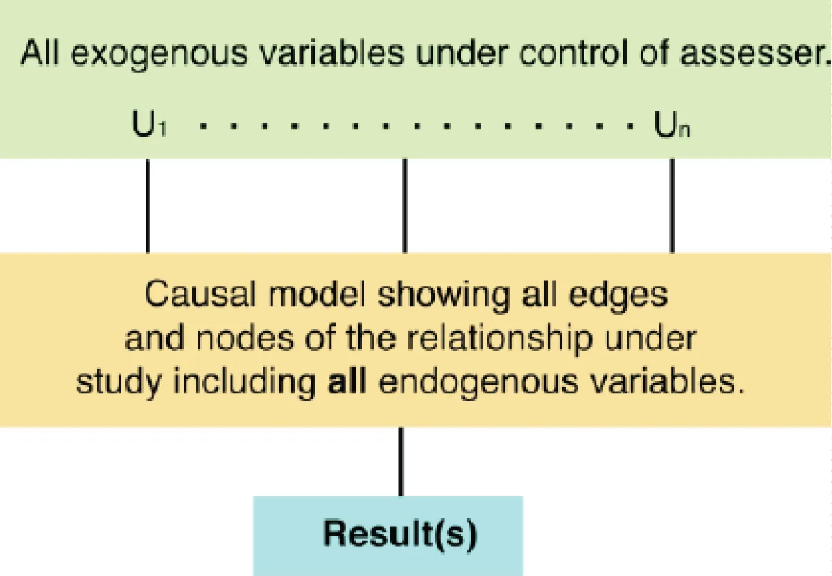
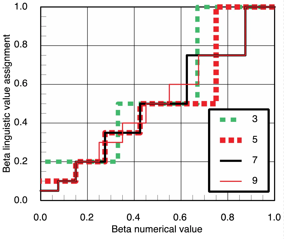
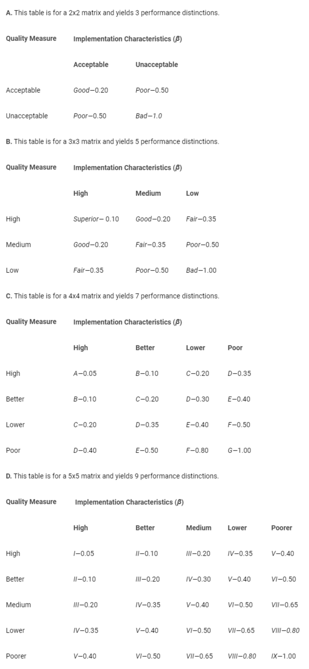
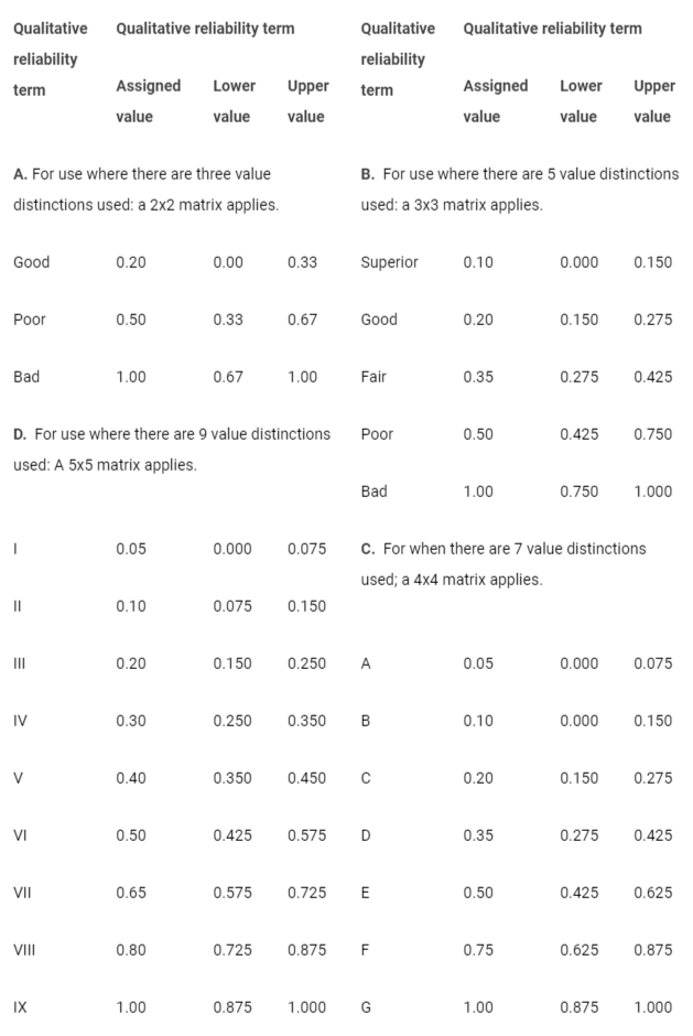
![<p>The following matrices for items 2 and 3 above describe the conditions that result in a Quality Assignment for the component under discussion based on the Quality Measure Characteristics and the Implementation Characteristics (how the information was evaluated by the assessor). With this pair of Quality Assignments for the Description and Implementation for a component, Table 2 provides the value for <em>b<sub>i</sub></em>. See Thiel, Zsutty, [13,17] for other examples for the other important issues considered.</p>](https://www.igminresearch.com/articles/fulltext/table_images/igmin111/Table3.png)