Improved Energy Valley Optimizer with Levy Flight for Optimization Problems

Abstract

Energy Valley Optimizer (EVO) is one of the recent metaheuristic algorithms. It draws inspiration from advanced principles in physics related to particle stability and decay modes. This paper presents a new Energy Valley Optimizer (EVO) and levy flights that are hybrid to improve the EVO in solving optimization problems. Levy flight is one of the most important randomization techniques. Fifteen mathematical test functions (five unimodal functions, four multimodal functions, and six composite functions) are solved with the proposed algorithm. We also compare our results with previous results of metaheuristic algorithms. The statistical results show that the results of the Levy Energy Valley Optimizer (LEVO) outperform other algorithms in almost all mathematical test functions.

Introduction

Optimization algorithms may be divided into two categories: deterministic and stochastic algorithms. Deterministic algorithms don’t contain stochastic operators; they give the same answer if the initial start point is constant. On the contrary, stochastic algorithms give different answers even if the initial start point is constant [1]. Metaheuristic algorithms are the most popular techniques for solving optimization problems. Natural phenomena inspire it. Such algorithms improved local optima solutions to reach global optima in search space [2]. The interested metaheuristic algorithms in the literature are Genetic Algorithms (GA) [3], Ant Colony Optimization (ACO) [4], Particle Swarm Optimization(PSO) [5], Artificial Bee Colony (ABC) Algorithm[6], Cuckoo Optimization Algorithm (COA) [7], Firefly Algorithm (FA) [8], Grey Wolf Optimizer (GWO) [9], Equilibrium optimizer (EO) [10], Horse herd optimization algorithm (HOA) [11], drawer algorithm (DA) [12], Walrus Optimization Algorithm (WaOA) [13], and Energy Valley Optimizer (EVO). The EVO is considered one of the latest nature-inspired algorithms proposed in metaheuristic algorithms [1]. The Energy Valley Optimizer (EVO) [1] is a recently developed metaheuristic algorithm that draws inspiration from sophisticated ideas in physics pertaining to particle stability and decay modes. The idea of the EVO comes from the fundamental laws of how particles decay through different types of matter in physics. The Energy Valley Optimizer also includes an examination of the complexity of the test functions used and achieves excellent results. As mentioned before, metaheuristics have shown a positive influence on feature selection problems in recent years [14]. There is still a need for additional optimization strategies to achieve further improved results. Exploration means finding promising solutions by seeking various unknown regions, while exploitation improves over solutions obtained by exploration [15].

Levy flight is a class of random walks whose step lengths are not constant but are drawn from levy distribution, proposed by Paul Levy [16]. The foraging movements are observed to follow Levy distribution. Levy flight makes a large jump in random walks, and this allows the individual to visit new sites that the swarm has not visited, which leads to high exploration in search space [17,18].

So, this paper presents a new Energy Valley Optimizer (EVO) and levy flights that are hybrid to improve the EVO in solving optimization problems. The remainder of the paper is organized as follows: in section 2, the basic EVO is described in detail. The definition of Levy flight and Levy Energy Valley optimizer (LEVO) algorithm is presented in section 3. Section 4 gives the experimental results. Finally, section 5 provides the conclusions of this work.

Overview of the basic EVO

Main inspiration: The Energy Valley Optimizer (EVO) [1] is a new metaheuristic algorithm that has been utilized in engineering optimization issues. It is classified within the category of physics-based approaches. EVO is inspired by the fundamental laws of how particles decay through different types of matter in physics. The term “physical reaction” pertains to the process of inducing the collision of two particles or foreign subatomic particles, resulting in the formation of novel particles. It is thought that most particles are unstable, but some are stable and stay that way forever. The unstable particles give off energy when they break apart, which is also known as decay. The total decay rate is different for each type of particle. During the decay process, a particle undergoes a reduction in energy, with the surplus energy being emitted. The Energy Valley concept involves scrutinizing particle stability by analyzing binding energy and how the particles interact with each other. The central focus in this domain centers on determining particle stability, which is contingent on evaluating neutron (N) and proton (Z) quantities, as well as the N/Z ratio. An N/Z ratio approximately equal to 1 signifies the particle is stable and light, whereas a higher N/Z value indicates stability in a heavier particle. Particles tend to enhance their stability by adjusting their neutron-to-proton (N/Z) ratio, gravitating towards the region of stability or the energy minimum, as illustrated in Figure 1A.

During the decay process, the emission of excessive energy results in the generation of a particle in a reduced energy state. The decay mechanism in particles exhibiting varying degrees of stability is determined by three distinct types of emissions. The alpha (α) particles are highly dense particles with a positive charge. Beta (β) particles are electrically charged particles that possess a negative charge. These particles can be described as electrons that exhibit greater velocities. Gamma (γ) rays are photons characterized by elevated energy levels, as deP_icted in Figure 1B. Based on the information provided regarding the emission process, it can be observed that there exist three distinct forms of decay, namely alpha, beta, and gamma decay, which are generated from the aforementioned emission kinds. Alpha decay is characterized by the emission of an alpha particle, leading to a decrease in both the neutron (N) and proton (Z) values and consequently reducing the N/Z ratio. Conversely, beta decay involves the emission of a β particle, posing a challenge to the N/Z ratio by reducing the number of neutrons (N) and increasing the number of protons (Z).In the process of gamma decay, the emission of a gamma (γ) photon from an excited particle is observed without any accompanying alteration in the N/Z values, as shown in Figure 1C. The EVO depends on the idea that different particles decay over time. The method uses the particles’ tendency to reach a stable point as a starting point for improving the performance of the candidate solutions.

Mathematical formula: The first phase involves the execution of the initialization procedure, during which the solution candidates (P_i) are conceptualized as particles that have varying degrees of stability inside the search space.

$\text{P}=\left[\begin{array}{c}{\text{P}}_1\\ {\text{P}}_2\\ ⋮\\ {\text{P}}_{\text{i}}\\ ⋮\\ {\text{P}}_{\text{n}}\end{array}\right]=\left[\begin{array}{c}{\text{p}}_1^1{\text{p}}_1^2\cdots {\text{p}}_1^{\text{j}}\cdots {\text{p}}_1^{\text{d}}\\ {\text{p}}_2^1{\text{p}}_2^2\cdots {\text{p}}_2^{\text{j}}\cdots {\text{p}}_2^{\text{d}}\\ \cdots \cdot \ddots \\ \cdots \\ {\text{p}}_i^1{\text{p}}_i^2\cdots {\text{p}}_i^{\text{j}}\cdots {\text{p}}_i^{\text{d}}\\ \cdots \cdot ⋮\\ {\text{p}}_{\text{n}}^1{\text{p}}_{\text{n}}^2\cdots {\text{p}}_{\text{n}}^{\text{j}}\cdots {\text{p}}_{\text{n}}^{\text{d}}\end{array}\right],\{\begin{array}{c}i=1,2,\dots ,n.\\ j=1,2,\dots ,d.\end{array}$ (1)

${\text{p}}_{\text{i}}^{\text{j}}={\text{p}}_{\text{i}, min }^{\text{j}}+\text{rand}\cdot \left({\text{p}}_{\text{i}, max }^{\text{j}}-{\text{p}}_{\text{i}, min }^{\text{j}}\right),\{\begin{array}{c}i=1,2,\dots ,n.\\ j=1,2,\dots ,d.\end{array}$ (2)

The variable “n” represents the particle number within the search space. The variable “d” represents the problem dimension under consideration. ${\text{p}}_{\text{i}}^{\text{j}}$ represents the j-th decision variable used to estimate the initial position of the i-th candidate. ${\text{ p}}_{\text{i}, max }^{\text{j}}$ and ${\text{p}}_{\text{i}, min }^{\text{j}}$ are the upper and lower bounds of the j-th variable in the i-th candidate. The variable “rand” represents a random number that follows a uniform distribution inside the interval [0,1].

The second phase of the method involves determining the Enrichment Bound (EB) for the particles. This parameter is employed to accommodate variations between particles with a surplus of neutrons and particles with a deficit of neutrons. In order to accomplish this, the evaluation function is assessed for every particle, leading to the determination of the Neutron Enrichment Level (NEL) of these particles. The aforementioned elements are mathematically represented in the following manner:

$\text{EB}=\frac{{\displaystyle {\sum }_{\text{i}=1}^n{\text{NEL}}_{\text{i}}}}{\text{n}}, \text{i}=1,2,\dots ,\text{n}.$ (3)

The variable NEL_i represents a level of neutron enrichment for the i-th particle, while EB denotes particles that are the enrichment bound.

In the third phase, the estimation of particle stability values is conducted by evaluating the objective function.

${\text{SL}}_{\text{i}}=\frac{{\text{NEL}}_{\text{i}}-\text{BS}}{\text{WS}-\text{BS}},\text{ i}=1,2,\dots ,\text{n}.$ (4)

The stability value for the i-th particle is SL_i, is determined based on the best (BS) and worst (WS) stability levels. These levels correspond to the lowest and highest objective function values discovered thus far. In the EVO’s main search loop, if a particle’s neutron enrichment level NEL_i surpasses the enrichment limit (EB), which implies that the particle has a higher neutron-to-proton (N/Z) ratio. Furthermore, alpha and gamma decays are anticipated to occur if the particle›s stability level SL_i exceeds the stability bound (SB). This expectation stems from the likelihood of such decay in larger particles with elevated stability levels. In the physics of alpha decay (as illustrated in Figure 2). The decision variables present in the solution candidate are substituted by the rays within the particle or candidate exhibiting the highest level of stability, referred to as S_BS. The mathematical representation of these is as follows:

${\text{P}}_{\text{i}}^{New1 }={\text{P}}_{\text{i}}\left({\text{P}}_{\text{BS}}\left({\text{p}}_{\text{i}}^{\text{j}}\right)\right), \{\begin{array}{c}i=1,2,\dots ,n.\\ j= Alpha Index II.\end{array}$ (5)

Where ${\text{P}}_{\text{i}}^{New1 }$ represents a newly produced particle within the search space, P_i is the current position vector of an i-th particle in search space. S_BS is the particle’s position vector that has the highest level of stability, ${\text{p}}_{\text{i}}^{\text{j}}$ is the j-th decision variable.

In this context, the estimation of the total distance between the particle under consideration and other particles is performed using a method, and the nearest particle is selected for this purpose.

${\text{D}}_{\text{i}}^{\text{k}}=\sqrt{{\left({\text{x}}_2-{\text{x}}_1\right)}^2+{\left({\text{y}}_2-{\text{y}}_1\right)}^2},\{\begin{array}{c}i=1,2,\dots ,n.\\ k=1,2,\dots ,n-1.\end{array}$ (6)

The variable ${\text{D}}_{\text{i}}^{\text{k}}$ represents the overall distance separating the i-th particle from the k-th neighboring particle. The coordinates of the particles are denoted by (x1, y1) and (x2, y2).

The procedure of updating the position to generate the second solution candidate in this phase is carried out by employing the following actions:

(7)

${\text{P}}_{\text{i}}^{New2 }$ is a newly generated particle

P_i is the current position vector of the i-th particle

P_Ng is the position vector of the neighboring particle around the i-th particle ${\text{p}}_{\text{i}}^{\text{j}}$ ​ is the j-th decision variable or emitted ray.

Beta decay takes place in particles with lower stability levels, indicating less stability. According to the principles of physics for beta decay, illustrated in Figure 2, particles release β rays to enhance their stability. Given the instability of these particles, a significant leap in the search space is necessary. In such cases, a procedure is employed to update the particle positions, involving controlled movements toward the particle or option with the best stability level (S_BS) and the center of the particles (P_CP). This aspect of the algorithm mimics the particles’ inclination to approach the stability band. Particles are situated near this band, and the majority of them exhibit higher stability (refer to Figure 1a and Figure 1b). These concepts are expressed as follows:

${\text{P}}_{\text{CP}}=\frac{{\displaystyle {\sum }_{i=1}^n}{\text{P}}_{\text{i}}}{\text{n}},i=1,2,\dots ,n.$ (8)

${\text{P}}_{\text{i}}^{\text{New}1}={\text{P}}_{\text{i}}+\frac{\left({\text{r}}_1\times {\text{P}}_{\text{BS}}-{\text{r}}_2\times {\text{P}}_{\text{CP}}\right)}{{\text{SL}}_{\text{i}}},\text{ i}=1,2,\dots ,\text{n}.$ (9)

${\text{P}}_{\text{i}}^{\text{New}1}$ the upcoming position vectors of i-th particles.

P_i the current position vectors of i-th particles.

S_BS is the particle position vector of the optimal stability level.

P_CP is the centre of the particle position vector

SL_i is the level of stability for the i-th particle.

The parameters r₁ and r₂ represent two randomly generated integers within the range of [0, 1].

To make the algorithm better at exploitation and exploration, a different process is used to update the positions of particles that use beta decay. This procedure entails guiding the particles systematically toward the particle with the optimal stability level (S_BS) and a neighboring particle or candidate (P_Ng), ensuring that the movement is not influenced by particle stability level. These elements can be mathematically articulated as follows:

${\text{P}}_{\text{i}}^{New2 }={\text{P}}_{\text{i}}+\left({\text{r}}_3\times {\text{P}}_{\text{BS}}-{\text{r}}_4\times {\text{P}}_{\text{Ng}}\right),\text{ i}=1,2,\dots ,\text{n}.$ (10)

${\text{P}}_{\text{i}}^{\text{New}2}$ is the forthcoming position vectors of i-th particles.

P_i is i-th particles’ current position vectors.

S_BS is the particle position vector of the optimal stability value.

PNg is the neighbouring particle’s position vector around the i-th particle.

The parameters r₃ and r₄ represent two randomly generated integers within the range of [0, 1].

When the neutron enrichment level (NEL_i) of a particle below the enrichment bound (EB), it is postulated that the particle possesses a reduced neutron-to-proton (N/Z) ratio. To approach the stability band, the particle has a tendency to either absorb electrons or emit positrons. In this context, a stochastic movement within the search space is characterized to accommodate these types of motions, expressed as follows:

${\text{P}}_{\text{i}}^{New }={\text{P}}_{\text{i}}+\text{r} , \text{i}=1,2,\dots ,\text{n}.$ (11)

where ${\text{P}}_{\text{i}}^{\text{New}}$ and P_i are the forthcoming and current position vectors of i-th particles.

The parameter r represents a randomly generated integer within the range of [0, 1].

Description Energy Valley Optimizer (LEVO)

Concept of levy flight: Levy flight is a kind of random walk whose step length is not constant, but it is drawn from levy distribution. Levy distribution has infinite variance and infinite mean with power low step size [19,20]. Some animals and insects, such as ants, are following levy flight in walk-in foraging patterns [21]. Levy distribution is useful for stochastic algorithms. It has a role in exploration and exploitation [22]. Levy flight is expressed mathematically as:

$levywalk=0.01\times \frac{x}{{\left|y\right|}^{\frac{1}{\beta }}}$ (12)

Where x and y are random numbers drawn from a normal distribution.

$x~N(0,{\sigma }_x^2),y~N(0,{\sigma }_y^2)$ (13)

Where ${\sigma }_x={\left(\frac{\Gamma (1+\beta )\times \sin (\frac{\pi \beta }{2})}{\Gamma (\frac{1+\beta }{2})\times \beta \times 2^{(\frac{\beta -1}{2})}}\right)}^{\raisebox{1ex}{$1$}\!\left/ \!\raisebox{-1ex}{$\beta $}\right.},{\sigma }_y=1, \Gamma \left(n\right)=\left(n-1\right)! \text{ and } 0<\beta \le 2,\beta =\raisebox{1ex}{$3$}\!\left/ \!\raisebox{-1ex}{$2$}\right.$

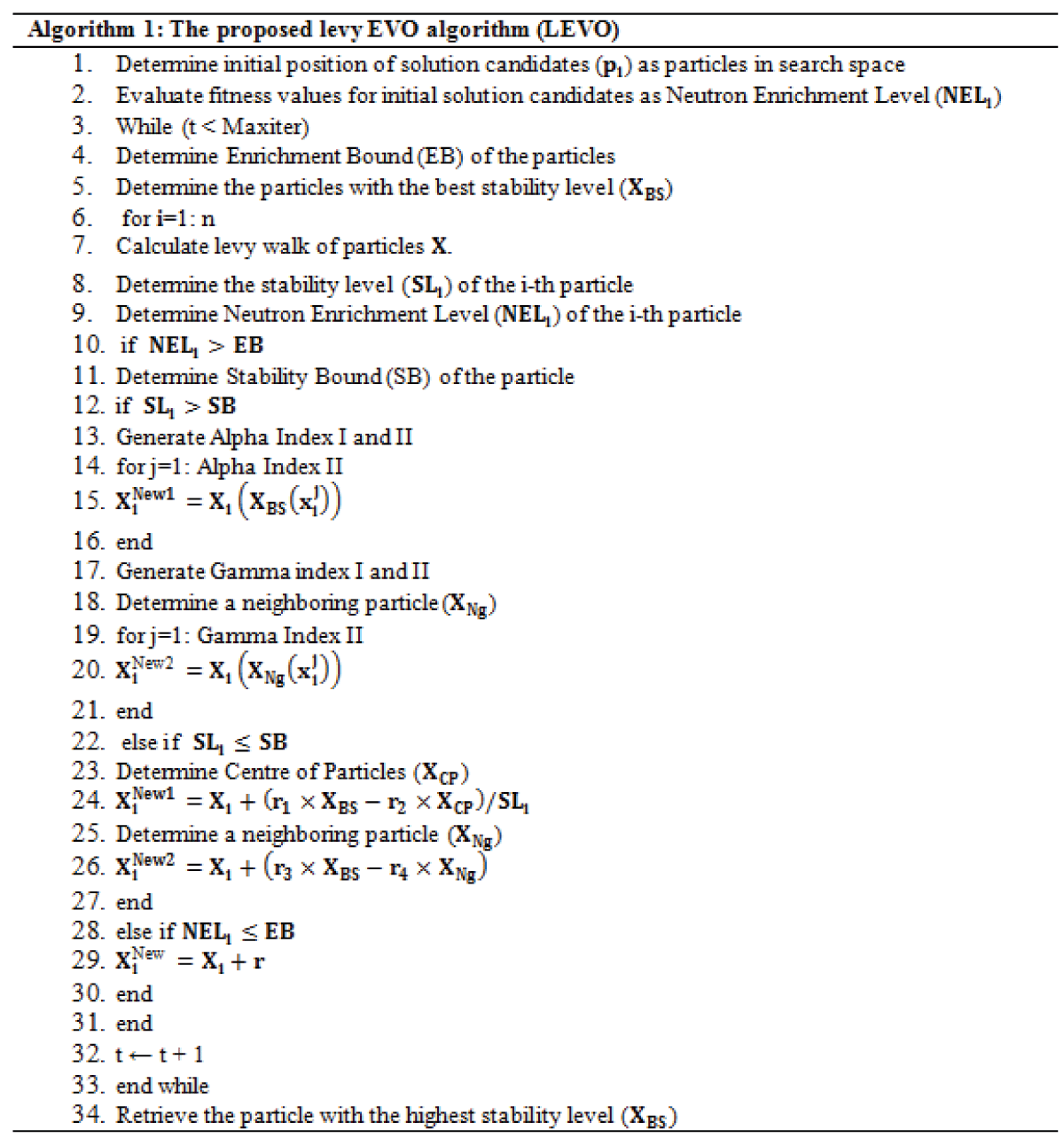
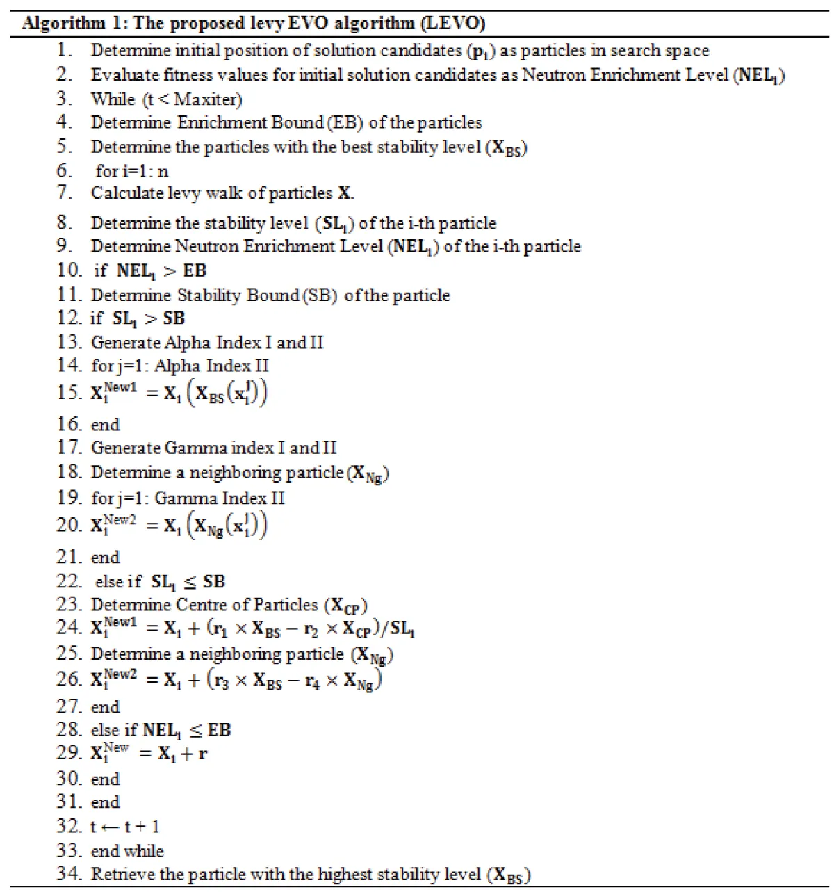
The proposed levy EVO algorithm (LEVO): The proposed (LEVO) is the improved form of the original EVO, where hybrid EVO with levy flight. In Algorithm 1, the proposed algorithm is represented in simple form.

Experimental results and discussions

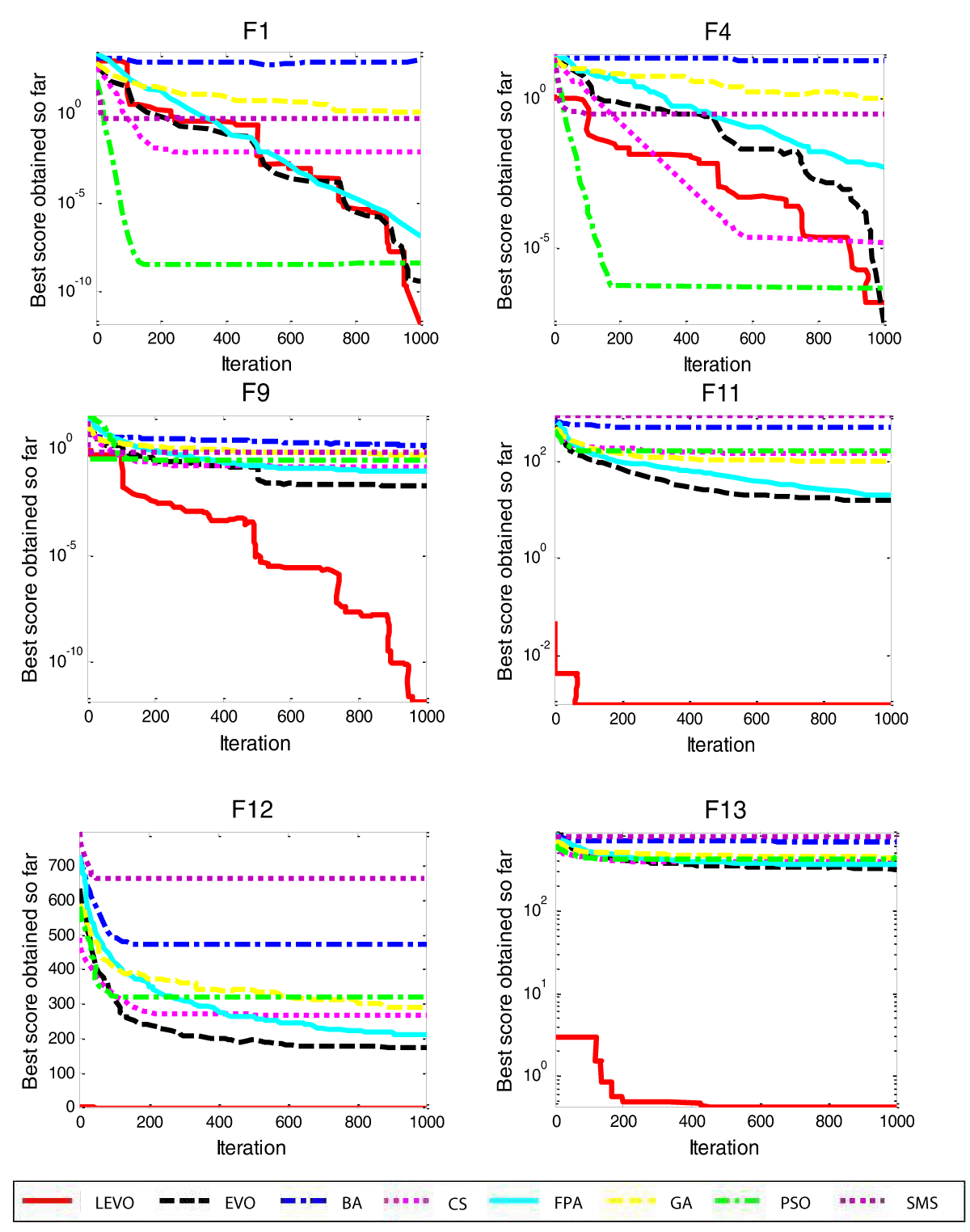
The results of fifteen benchmark functions are presented in this section. These test functions can be classified into three categories. The first category, unimodal test functions, contains five test functions. The second contains four functions of multimodal functions. The other six problems are composite test functions located in the last category. Tables 1-3 present the test function survey of each category. The proposed LEVO is compared with the basic Energy valley optimizer (EVO) [1] and recent algorithms such as Genetic Algorithms (GA) [3], Particle Swarm Optimization (PSO) [5], Firefly Algorithm (FA) [8], states of matter search (SMS) [23], Bat algorithm (BA) [24], Flower pollination algorithm (FPA) [25], and Cuckoo search (CS) [26]. The proposed LEVO algorithm uses 30 candidate solutions (particles) over 1000 iterations. For each category, two tables are given. The first table includes the values of the decision variable and the objective function of the best run out of 30 independent runs. The second table contains Ave and std. Ave is the mean of the optimal objective value calculated for 30 independent runs. Std is the standard deviation of optimal objective values Table 4.

Results on unimodal benchmark functions

The Unimodal function is the function that has a single optimum. Test functions are presented in Table 1. Table 5 presents the best values of objective functions among 30 independent runs and their corresponding decision variables (x’s). Statistical results are listed in Table 6. Results show that, on most test functions, the proposed LEVO algorithm gets better results than other algorithms.

Results on multimodal benchmark functions

The Multimodal function is a function that has more than one optimum in which there is a single global optimum. These test functions are presented in Table 2. Table 7 shows the results of the proposed LEVO on multimodal function; the average of the minimum value (ave) and their standard deviation (std) are presented in Table 8. It is clear that the LEVO algorithm has the best results in many test functions.

Results on composite benchmark functions

Composite benchmark functions are listed in Table 3. Table 9 shows the results of composite functions using LEVO. The average (Ave) and their standard deviation (std) are presented in Table 10. Results show that the proposed LEVO algorithm outperforms other algorithms on the majority of the test functions.

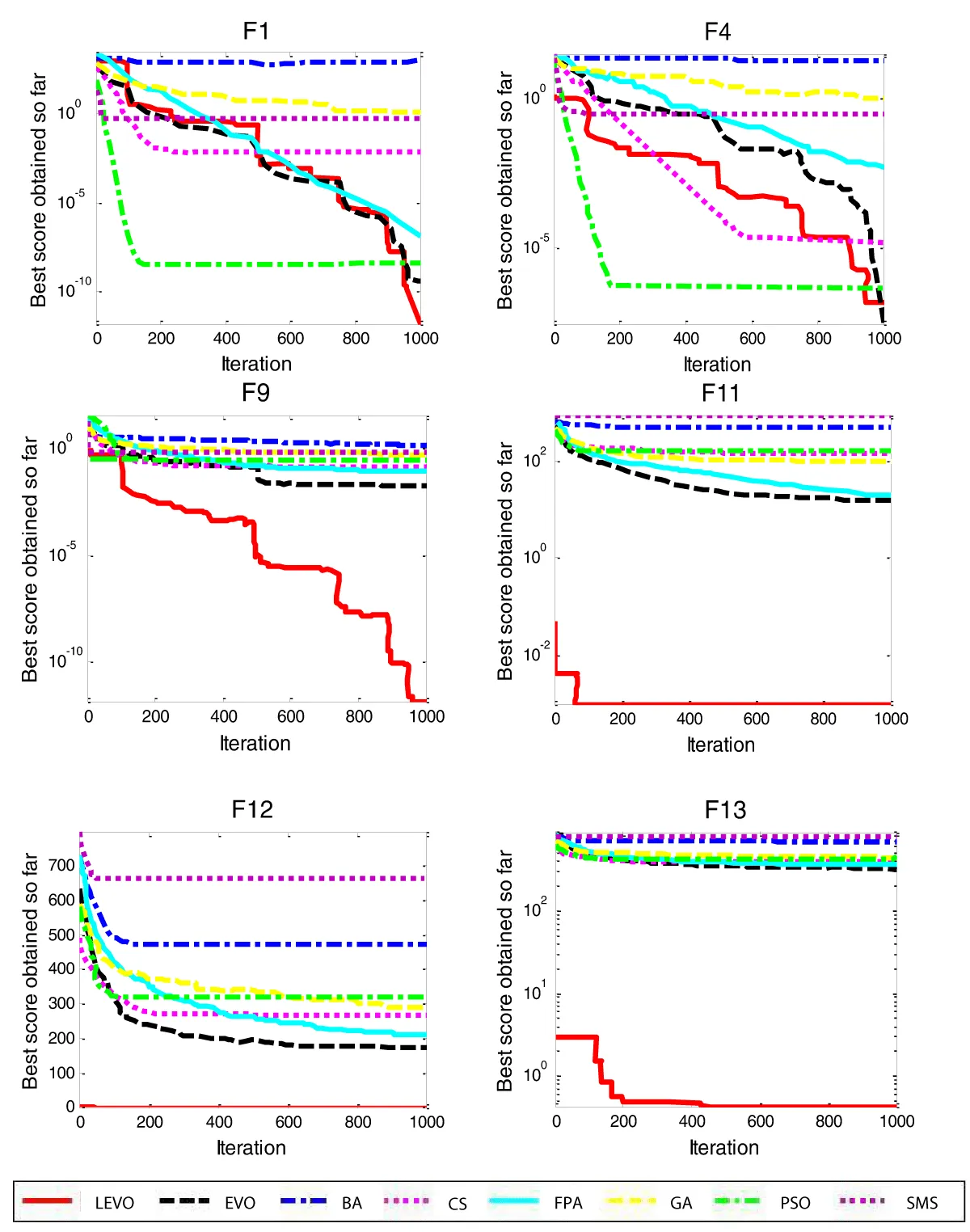
The convergence curves of algorithms on some of the test functions are illustrated in Figure 3.

Performance of LEVO in large-scale problems: To verify the performance of the proposed LEVO algorithm in large-scale optimization problems, this subsection solves the 200-dimensional versions of the unimodal and multimodal test functions. LEVO algorithm is tested with two cases of parameters, as illustrated in Table 11. Results of the proposed LEVO algorithm are compared with PSO, SMS, BA, FPA, CS, FA, GA, and classic EVO (search agent=100, 5000 iteration). The results of unimodal test functions are reported in Table 12, and multimodal test functions are presented in Table 13.

According to the results in Tables 12,13, it is clear that LEVO (case1, 2) outperforms all the other algorithms in the majority of test cases. Also, LEVO (case 1) gives almost the same result as LEVO (case 2) although the search agent and iteration become lesser. These results show that LEVO avoids local optima, and resolves local optima stagnation in solving the challenging problem because of using levy flight.

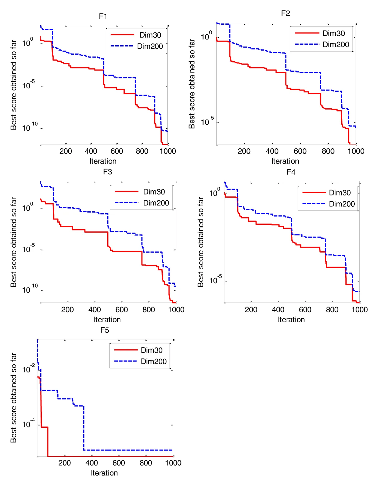
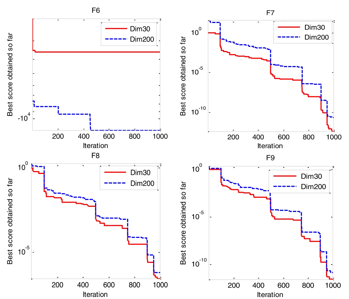
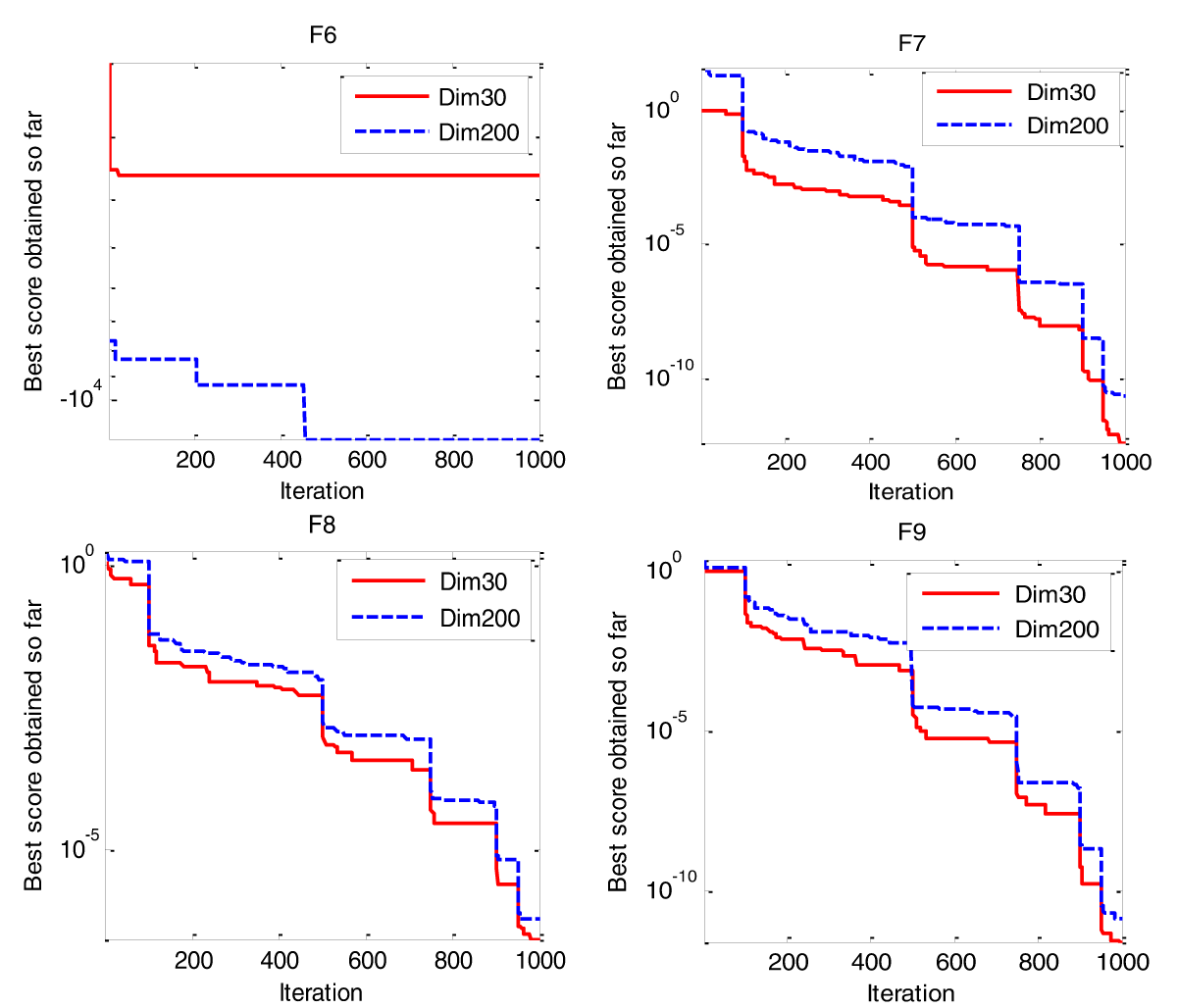
Figures 4,5 illustrate the behavior of LEVO in solving small and large dimensions (Dim=30, Dim=200). It is obvious that the convergence behavior is almost the same in the case of increasing dimensions (convergence to optimal occurs in the same iteration, although the increase of dimensions).

Conclusion

This work improved the behavior of a nature-inspired algorithm called EVO. This paper improves EVO by hybrid levy flight with the original EVO. Using levy flight has a better effect on the performance of the EVO algorithm, and this is because the levy walk makes a large jump of particles; this allows particles to Visit new sites, leads to local optima avoidance, and high exploration in search space. The proposed LEVO was benchmarked on fifteen test functions. These test functions are compared with algorithms described in the literature in terms of fitness improvement of the population, exploration, exploitation, and local optima avoidance. From the results, we can conclude that the proposed LEVO outperforms other algorithms on the majority of test functions. In addition, the performance of LEVO is tested in unimodal and multimodal large-scale problems. Results of EVO, GA, PSO, FA, SMS, BA, FPA, and CS (at a hundred search agents over 5,000 iterations) are compared with LEVO (at 30 search agents and 1,000 iterations). The results showed that LEVO outperforms all the other algorithms on the majority of test functions, although the search agent and iteration become less. Also, we can prove that the results of LEVO case 1 (30 search agents and 1000 iterations) give almost the same results as LEVO case 2 (at 100 search agents and 5000 iterations). Finally, we test the behavior of LEVO in small and large dimensions, and it turns out that the convergence behavior and convergence to optimal occur in the same iteration, although the dimensions increase. That makes us conclude that the proposed LEVO algorithm can be very effective for solving large-scale problems as well.

About the Article